The Machine Learning Library (MLL) is a set of classes and functions for statistical classification, regression and clustering of data.
Most of the classification and regression algorithms are implemented as C++ classes.
As the algorithms have different set of features (like ability to handle missing measurements,
or categorical input variables etc.), there is a little common ground between the classes.
This common ground is defined by the class CvStatModel that all
the other ML classes are derived from.
Base class for statistical models in ML
class CvStatModel
{
public:
    /* CvStatModel(); */
    /* CvStatModel( const CvMat* train_data ... ); */

    virtual ~CvStatModel();

    virtual void clear()=0;

    /* virtual bool train( const CvMat* train_data, [int tflag,] ..., const CvMat* responses, ...,
    [const CvMat* var_idx,] ..., [const CvMat* sample_idx,] ...
    [const CvMat* var_type,] ..., [const CvMat* missing_mask,] <misc_training_alg_params> ... )=0;
     */

    /* virtual float predict( const CvMat* sample ... ) const=0; */

    virtual void save( const char* filename, const char* name=0 )=0;
    virtual void load( const char* filename, const char* name=0 )=0;

    virtual void write( CvFileStorage* storage, const char* name )=0;
    virtual void read( CvFileStorage* storage, CvFileNode* node )=0;
};
In this declaration some methods are commented off. Actually, these are methods for which there is no unified API (with the exception of the default constructor), however, there are many similarities in the syntax and semantics that are briefly described below in this section, as if they are a part of the base class.
Default constructor
CvStatModel::CvStatModel();
Each statistical model class in ML has default constructor without parameters. This constructor is useful for 2-stage model construction, when the default constructor is followed by train() or load().
Training constructor
CvStatModel::CvStatModel( const CvMat* train_data ... ); */
Most ML classes provide single-step construct+train constructor. This constructor is equivalent to the default constructor, followed by the train() method with the parameters that passed to the constructor.
Virtual destructor
CvStatModel::~CvStatModel();
The destructor of the base class is declared as virtual, so it is safe to write the following code:
CvStatModel* model;
if( use_svm )
    model = new CvSVM(... /* SVM params */);
else
    model = new CvDTree(... /* Decision tree params */);
...
delete model;
Normally, the destructor of each derived class does nothing, but calls
the overridden method clear() that deallocates all the memory.
Deallocates memory and resets the model state
void CvStatModel::clear();
The method clear does the same job as the destructor, i.e. it deallocates all the memory
occupied by the class members. But the object itself is not destructed, and it can be reused further.
This method is called from the destructor, from the train methods of the derived classes,
from the methods load(),
read() etc., or even explicitly by user.
Saves the model to file
void CvStatModel::save( const char* filename, const char* name=0 );
The method save stores the complete model state to the specified XML or YAML file
with the specified name or default name (that depends on the particular class).
Data persistence
functionality from cxcore is used.
Loads the model from file
void CvStatModel::load( const char* filename, const char* name=0 );
The method load loads the complete model state with the specified
name
(or default model-dependent name) from the specified XML or YAML file. The
previous model state is cleared by clear().
Note that the method is virtual, therefore any model can be loaded using this virtual method. However, unlike the C types of OpenCV that can be loaded using generic cvLoad(), in this case the model type must be known anyway, because an empty model, an instance of the appropriate class, must be constructed beforehand. This limitation will be removed in the later ML versions.
Writes the model to file storage
void CvStatModel::write( CvFileStorage* storage, const char* name );
The method write stores the complete model state
to the file storage
with the specified name or default name (that depends on the particular class).
The method is called by save().
Reads the model from file storage
void CvStatMode::read( CvFileStorage* storage, CvFileNode* node );
The method read restores the complete model state from the specified node
of the file storage. The node must be located by user, for example, using
the function cvGetFileNodeByName().
The method is called by load().
The previous model state is cleared by clear().
Trains the model
bool CvStatMode::train( const CvMat* train_data, [int tflag,] ..., const CvMat* responses, ...,
    [const CvMat* var_idx,] ..., [const CvMat* sample_idx,] ...
    [const CvMat* var_type,] ..., [const CvMat* missing_mask,] <misc_training_alg_params> ... );
The method trains the statistical model using a set of input feature vectors and the corresponding
output values (responses). Both input and output vectors/values are passed as matrices.
By default the input feature vectors are stored as train_data rows,
i.e. all the components (features) of a training vector are stored
continuously. However, some algorithms can handle the transposed representation,
when all values of each particular feature (component/input variable)
over the whole input set are stored continuously. If both layouts are supported, the method
includes tflag parameter that specifies the orientation:
tflag=CV_ROW_SAMPLE means that the feature vectors are stored as rows,
tflag=CV_COL_SAMPLE means that the feature vectors are stored as columns.
The train_data must have
32fC1 (32-bit floating-point, single-channel) format.
Responses are usually stored in the 1d
vector (a row or a column) of 32sC1 (only in the classification problem) or
32fC1 format, one value per an input vector (although some algorithms, like various flavors of neural nets,
take vector responses).
For classification problems the responses are discrete class labels,
for regression problems - the responses are values of the function to be approximated.
Some algorithms can deal only with classification problems, some - only with regression problems,
and some can deal with both problems. In the latter case the type of output variable is either passed as separate parameter,
or as a last element of var_type vector:
CV_VAR_CATEGORICAL means that the output values are discrete class labels,
CV_VAR_ORDERED(=CV_VAR_NUMERICAL) means that the output values are ordered, i.e.
2 different values can be compared as numbers, and this is a regression problem
The types of input variables can be also specified using var_type.
Most algorithms can handle only ordered input variables.
Many models in the ML may be trained on a selected feature subset,
and/or on a selected sample subset of the training set. To make it easier for user,
the method train usually includes var_idx
and sample_idx parameters. The former identifies variables (features) of interest,
and the latter identifies samples of interest. Both vectors are either integer (32sC1)
vectors, i.e. lists of 0-based indices, or 8-bit (8uC1) masks of active variables/samples.
User may pass NULL pointers instead of either of the argument, meaning that
all the variables/samples are used for training.
Additionally some algorithms can handle missing measurements,
that is when certain features of
certain training samples have unknown values (for example, they forgot to
measure a temperature
of patient A on Monday). The parameter missing_mask, 8-bit matrix of the same size as
train_data, is used to mark the missed values (non-zero elements of the mask).
Usually, the previous model state is cleared by clear() before running the training procedure. However, some algorithms may optionally update the model state with the new training data, instead of resetting it.
Predicts the response for sample
float CvStatMode::predict( const CvMat* sample[, <prediction_params>] ) const;
The method is used to predict the response for a new sample. In case of
classification the method returns the class label, in case of regression - the
output function value. The input sample must have as many components as the
train_data passed to train
contains. If the var_idx parameter is passed to train,
it is remembered and then is used to extract only the necessary components from the input sample
in the method predict.
The suffix "const" means that prediction does not affect the internal model state, so the method can be safely called from within different threads.
[Fukunaga90] K. Fukunaga. Introduction to Statistical Pattern Recognition. second ed., New York: Academic Press, 1990.
Bayes classifier for normally distributed data
class CvNormalBayesClassifier : public CvStatModel
{
public:
    CvNormalBayesClassifier();
    virtual ~CvNormalBayesClassifier();

    CvNormalBayesClassifier( const CvMat* _train_data, const CvMat* _responses,
        const CvMat* _var_idx=0, const CvMat* _sample_idx=0 );

    virtual bool train( const CvMat* _train_data, const CvMat* _responses,
        const CvMat* _var_idx = 0, const CvMat* _sample_idx=0, bool update=false );

    virtual float predict( const CvMat* _samples, CvMat* results=0 ) const;
    virtual void clear();

    virtual void save( const char* filename, const char* name=0 );
    virtual void load( const char* filename, const char* name=0 );

    virtual void write( CvFileStorage* storage, const char* name );
    virtual void read( CvFileStorage* storage, CvFileNode* node );
protected:
    ...
};
Trains the model
bool CvNormalBayesClassifier::train( const CvMat* _train_data, const CvMat* _responses,
               const CvMat* _var_idx = 0, const CvMat* _sample_idx=0, bool update=false );
The method trains the Normal Bayes classifier. It follows the conventions of
generic train "method" with the following limitations:
only CV_ROW_SAMPLE data layout is supported; the input variables are all ordered;
the output variable is categorical (i.e. elements of _responses
must be integer numbers, though the vector may have 32fC1 type),
missing measurements are not supported.
In addition, there is update flag that identifies, whether the model should
be trained from scratch (update=false) or should be updated using new training data
(update=true).
Predicts the response for sample(s)
float CvNormalBayesClassifier::predict( const CvMat* samples, CvMat* results=0 ) const;
The method predict estimates the most probable classes for the input vectors.
The input vectors (one or more) are stored as rows of the matrix samples.
In case of multiple input vectors, there should be output vector results.
The predicted class for a single input vector is returned by the method.
The algorithm caches all the training samples, and it predicts the response for a new sample by analyzing a certain number (K) of the nearest neighbors of the sample (using voting, calculating weighted sum etc.) The method is sometimes referred to as "learning by example", i.e. for prediction it looks for the feature vector with a known response that is closest to the given vector.
K Nearest Neighbors model
class CvKNearest : public CvStatModel
{
public:

    CvKNearest();
    virtual ~CvKNearest();

    CvKNearest( const CvMat* _train_data, const CvMat* _responses,
                const CvMat* _sample_idx=0, bool _is_regression=false, int max_k=32 );

    virtual bool train( const CvMat* _train_data, const CvMat* _responses,
                        const CvMat* _sample_idx=0, bool is_regression=false,
                        int _max_k=32, bool _update_base=false );

    virtual float find_nearest( const CvMat* _samples, int k, CvMat* results,
        const float** neighbors=0, CvMat* neighbor_responses=0, CvMat* dist=0 ) const;

    virtual void clear();
    int get_max_k() const;
    int get_var_count() const;
    int get_sample_count() const;
    bool is_regression() const;

protected:
    ...
};
Trains the model
bool CvKNearest::train( const CvMat* _train_data, const CvMat* _responses,
                        const CvMat* _sample_idx=0, bool is_regression=false,
                        int _max_k=32, bool _update_base=false );
The method trains the K-Nearest model. It follows the conventions of
generic train "method" with the following limitations:
only CV_ROW_SAMPLE data layout is supported, the input variables are all ordered,
the output variables can be either categorical (is_regression=false)
or ordered (is_regression=true), variable subsets (var_idx) and
missing measurements are not supported.
The parameter _max_k specifies the number of maximum neighbors that may be
passed to the method find_nearest.
The parameter _update_base specifies, whether the model is trained from scratch (_update_base=false), or
it is updated using the new training data
(_update_base=true). In the latter case the parameter _max_k
must not be larger than the original value.
Finds the neighbors for the input vectors
float CvKNearest::find_nearest( const CvMat* _samples, int k, CvMat* results=0,
        const float** neighbors=0, CvMat* neighbor_responses=0, CvMat* dist=0 ) const;
For each input vector (which are rows of the matrix _samples)
the method finds k≤get_max_k() nearest neighbor. In case of regression,
the predicted result will be a mean value of the particular vector's neighbor responses.
In case of classification the class is determined by voting.
For custom classification/regression prediction, the method can optionally return
pointers to the neighbor vectors themselves (neighbors, array of
k*_samples->rows pointers), their corresponding output values
(neighbor_responses, a vector of k*_samples->rows elements)
and the distances from the input vectors to the neighbors
(dist, also a vector of k*_samples->rows elements).
For each input vector the neighbors are sorted by their distances to the vector.
If only a single input vector is passed, all output matrices are optional and the predicted value is returned by the method.
#include "ml.h"
#include "highgui.h"

int main( int argc, char** argv )
{
    const int K = 10;
    int i, j, k, accuracy;
    float response;
    int train_sample_count = 100;
    CvRNG rng_state = cvRNG(-1);
    CvMat* trainData = cvCreateMat( train_sample_count, 2, CV_32FC1 );
    CvMat* trainClasses = cvCreateMat( train_sample_count, 1, CV_32FC1 );
    IplImage* img = cvCreateImage( cvSize( 500, 500 ), 8, 3 );
    float _sample[2];
    CvMat sample = cvMat( 1, 2, CV_32FC1, _sample );
    cvZero( img );

    CvMat trainData1, trainData2, trainClasses1, trainClasses2;

    // form the training samples
    cvGetRows( trainData, &trainData1, 0, train_sample_count/2 );
    cvRandArr( &rng_state, &trainData1, CV_RAND_NORMAL, cvScalar(200,200), cvScalar(50,50) );

    cvGetRows( trainData, &trainData2, train_sample_count/2, train_sample_count );
    cvRandArr( &rng_state, &trainData2, CV_RAND_NORMAL, cvScalar(300,300), cvScalar(50,50) );

    cvGetRows( trainClasses, &trainClasses1, 0, train_sample_count/2 );
    cvSet( &trainClasses1, cvScalar(1) );

    cvGetRows( trainClasses, &trainClasses2, train_sample_count/2, train_sample_count );
    cvSet( &trainClasses2, cvScalar(2) );

    // learn classifier
    CvKNearest knn( trainData, trainClasses, 0, false, K );
    CvMat* nearests = cvCreateMat( 1, K, CV_32FC1);

    for( i = 0; i < img->height; i++ )
    {
        for( j = 0; j < img->width; j++ )
        {
            sample.data.fl[0] = (float)j;
            sample.data.fl[1] = (float)i;

            // estimates the response and get the neighbors' labels
            response = knn.find_nearest(&sample,K,0,0,nearests,0);

            // compute the number of neighbors representing the majority
            for( k = 0, accuracy = 0; k < K; k++ )
            {
                if( nearests->data.fl[k] == response)
                    accuracy++;
            }
            // highlight the pixel depending on the accuracy (or confidence)
            cvSet2D( img, i, j, response == 1 ?
                (accuracy > 5 ? CV_RGB(180,0,0) : CV_RGB(180,120,0)) :
                (accuracy > 5 ? CV_RGB(0,180,0) : CV_RGB(120,120,0)) );
        }
    }

    // display the original training samples
    for( i = 0; i < train_sample_count/2; i++ )
    {
        CvPoint pt;
        pt.x = cvRound(trainData1.data.fl[i*2]);
        pt.y = cvRound(trainData1.data.fl[i*2+1]);
        cvCircle( img, pt, 2, CV_RGB(255,0,0), CV_FILLED );
        pt.x = cvRound(trainData2.data.fl[i*2]);
        pt.y = cvRound(trainData2.data.fl[i*2+1]);
        cvCircle( img, pt, 2, CV_RGB(0,255,0), CV_FILLED );
    }

    cvNamedWindow( "classifier result", 1 );
    cvShowImage( "classifier result", img );
    cvWaitKey(0);

    cvReleaseMat( &trainClasses );
    cvReleaseMat( &trainData );
    return 0;
}
Originally, support vector machines (SVM) was a technique for building an optimal (in some sense) binary (2-class) classifier. Then the technique has been extended to regression and clustering problems. SVM is a partial case of kernel-based methods, it maps feature vectors into higher-dimensional space using some kernel function, and then it builds an optimal linear discriminating function in this space (or an optimal hyperplane that fits into the training data, ...). In case of SVM the kernel is not defined explicitly. Instead, a distance between any 2 points in the hyperspace needs to be defined.
The solution is optimal in a sense that the margin between the separating hyperplane and the nearest feature vectors from the both classes (in case of 2-class classifier) is maximal. The feature vectors that are the closest to the hyperplane are called "support vectors", meaning that the position of other vectors does not affect the hyperplane (the decision function).
There are a lot of good references on SVM. Here are only a few ones to start with.
[Burges98] C. Burges. "A tutorial on support vector machines for pattern recognition", Knowledge Discovery and Data Mining 2(2), 1998.Support Vector Machines
class CvSVM : public CvStatModel
{
public:
    // SVM type
    enum { C_SVC=100, NU_SVC=101, ONE_CLASS=102, EPS_SVR=103, NU_SVR=104 };

    // SVM kernel type
    enum { LINEAR=0, POLY=1, RBF=2, SIGMOID=3 };

    CvSVM();
    virtual ~CvSVM();

    CvSVM( const CvMat* _train_data, const CvMat* _responses,
           const CvMat* _var_idx=0, const CvMat* _sample_idx=0,
           CvSVMParams _params=CvSVMParams() );

    virtual bool train( const CvMat* _train_data, const CvMat* _responses,
                        const CvMat* _var_idx=0, const CvMat* _sample_idx=0,
                        CvSVMParams _params=CvSVMParams() );

    virtual float predict( const CvMat* _sample ) const;
    virtual int get_support_vector_count() const;
    virtual const float* get_support_vector(int i) const;
    virtual void clear();

    virtual void save( const char* filename, const char* name=0 );
    virtual void load( const char* filename, const char* name=0 );

    virtual void write( CvFileStorage* storage, const char* name );
    virtual void read( CvFileStorage* storage, CvFileNode* node );
    int get_var_count() const { return var_idx ? var_idx->cols : var_all; }

protected:
    ...
};
SVM training parameters
struct CvSVMParams
{
    CvSVMParams();
    CvSVMParams( int _svm_type, int _kernel_type,
                 double _degree, double _gamma, double _coef0,
                 double _C, double _nu, double _p,
                 CvMat* _class_weights, CvTermCriteria _term_crit );

    int         svm_type;
    int         kernel_type;
    double      degree; // for poly
    double      gamma;  // for poly/rbf/sigmoid
    double      coef0;  // for poly/sigmoid

    double      C;  // for CV_SVM_C_SVC, CV_SVM_EPS_SVR and CV_SVM_NU_SVR
    double      nu; // for CV_SVM_NU_SVC, CV_SVM_ONE_CLASS, and CV_SVM_NU_SVR
    double      p; // for CV_SVM_EPS_SVR
    CvMat*      class_weights; // for CV_SVM_C_SVC
    CvTermCriteria term_crit; // termination criteria
};
C for outliers.nu
(in the range 0..1, the larger the value, the smoother the decision boundary) is used instead of C.p. For outliers
the penalty multiplier C is used.nu is used instead of p.
C and thus affect the misclassification penalty for different classes.
The larger weight, the larger penalty on misclassification of data from the corresponding class.
The structure must be initialized and passed to the training method of CvSVM
Trains SVM
bool CvSVM::train( const CvMat* _train_data, const CvMat* _responses,
                   const CvMat* _var_idx=0, const CvMat* _sample_idx=0,
                   CvSVMParams _params=CvSVMParams() );
The method trains the SVM model. It follows the conventions of
generic train "method" with the following limitations:
only CV_ROW_SAMPLE data layout is supported, the input variables are all ordered,
the output variables can be either categorical (_params.svm_type=CvSVM::C_SVC or
_params.svm_type=CvSVM::NU_SVC), or ordered
(_params.svm_type=CvSVM::EPS_SVR or
_params.svm_type=CvSVM::NU_SVR), or not required at all
(_params.svm_type=CvSVM::ONE_CLASS),
missing measurements are not supported.
All the other parameters are gathered in CvSVMParams structure.
Retrieves the number of support vectors and the particular vector
int CvSVM::get_support_vector_count() const;
const float* CvSVM::get_support_vector(int i) const;
The methods can be used to retrieve the set of support vectors.
The ML classes discussed in this section implement Classification And Regression Tree algorithms, which is described in [Brieman84].
The class CvDTree represents a single decision tree that may be used alone, or as a base class in tree ensembles (see Boosting and Random Trees).
Decision tree is a binary tree (i.e. tree where each non-leaf node has exactly 2 child nodes). It can be used either for classification, when each tree leaf is marked with some class label (multiple leafs may have the same label), or for regression, when each tree leaf is also assigned a constant (so the approximation function is piecewise constant).
To reach a leaf node, and thus to obtain a response for the input feature vector, the prediction procedure starts with the root node. From each non-leaf node the procedure goes to the left (i.e. selects the left child node as the next observed node), or to the right based on the value of a certain variable, which index is stored in the observed node. The variable can be either ordered or categorical. In the first case, the variable value is compared with the certain threshold (which is also stored in the node); if the value is less than the threshold, the procedure goes to the left, otherwise, to the right (for example, if the weight is less than 1 kilo, the procedure goes to the left, else to the right). And in the second case the discrete variable value is tested, whether it belongs to a certain subset of values (also stored in the node) from a limited set of values the variable could take; if yes, the procedure goes to the left, else - to the right (for example, if the color is green or red, go to the left, else to the right). That is, in each node, a pair of entities (<variable_index>, <decision_rule (threshold/subset)>) is used. This pair is called split (split on the variable #<variable_index>). Once a leaf node is reached, the value assigned to this node is used as the output of prediction procedure.
Sometimes, certain features of the input vector are missed (for example, in the darkness it is difficult to determine the object color), and the prediction procedure may get stuck in the certain node (in the mentioned example if the node is split by color). To avoid such situations, decision trees use so-called surrogate splits. That is, in addition to the best "primary" split, every tree node may also be split on one or more other variables with nearly the same results.
The tree is built recursively, starting from the root node. The whole training data (feature
vectors and the responses) are used to split the root node. In each node the optimum
decision rule (i.e. the best "primary" split) is found based on some criteria (in ML gini "purity" criteria is used
for classification, and sum of squared errors is used for regression). Then, if necessary,
the surrogate
splits are found that resemble at the most the results of the primary split on
the training data; all data are divided using the primary and the surrogate splits
(just like it is done in the prediction procedure)
between the left and the right child node. Then the procedure recursively splits both left and right
nodes etc. At each node the recursive procedure may stop (i.e. stop splitting the node further)
in one of the following cases:
When the tree is built, it may be pruned using cross-validation procedure, if need. That is, some branches of the tree that may lead to the model overfitting are cut off. Normally, this procedure is only applied to standalone decision trees, while tree ensembles usually build small enough trees and use their own protection schemes against overfitting.
Besides the obvious use of decision trees - prediction, the tree can be also used for various data analysis. One of the key properties of the constructed decision tree algorithms is that it is possible to compute importance (relative decisive power) of each variable. For example, in a spam filter that uses a set of words occurred in the message as a feature vector, the variable importance rating can be used to determine the most "spam-indicating" words and thus help to keep the dictionary size reasonable.
Importance of each variable is computed over all the splits on this variable in the tree, primary and surrogate ones. Thus, to compute variable importance correctly, the surrogate splits must be enabled in the training parameters, even if there is no missing data.
Decision tree node split
struct CvDTreeSplit
{
    int var_idx;
    int inversed;
    float quality;
    CvDTreeSplit* next;
    union
    {
        int subset[2];
        struct
        {
            float c;
            int split_point;
        }
        ord;
    };
};
if var_value in subset then next_node<-left else next_node<-right
if var_value < c then next_node<-left else next_node<-right
Decision tree node
struct CvDTreeNode
{
    int class_idx;
    int Tn;
    double value;

    CvDTreeNode* parent;
    CvDTreeNode* left;
    CvDTreeNode* right;

    CvDTreeSplit* split;

    int sample_count;
    int depth;
    ...
};
Tn
of the whole tree, child nodes have Tn less than or equal to
the parent's Tn,
and the nodes with Tn≤CvDTree::pruned_tree_idx are not taken
into consideration at the prediction stage (the corresponding branches are
considered as cut-off), even
if they have not been physically deleted from the tree at the pruning stage.
left->sample_count>right->sample_count and
to the right otherwise.
Other numerous fields of CvDTreeNode are used internally at the training stage.
Decision tree training parameters
struct CvDTreeParams
{
    int max_categories;
    int max_depth;
    int min_sample_count;
    int cv_folds;
    bool use_surrogates;
    bool use_1se_rule;
    bool truncate_pruned_tree;
    float regression_accuracy;
    const float* priors;

    CvDTreeParams() : max_categories(10), max_depth(INT_MAX), min_sample_count(10),
        cv_folds(10), use_surrogates(true), use_1se_rule(true),
        truncate_pruned_tree(true), regression_accuracy(0.01f), priors(0)
    {}

    CvDTreeParams( int _max_depth, int _min_sample_count,
                   float _regression_accuracy, bool _use_surrogates,
                   int _max_categories, int _cv_folds,
                   bool _use_1se_rule, bool _truncate_pruned_tree,
                   const float* _priors );
};
max_depth. The actual depth
may
be smaller if the other termination criteria are met
(see the outline of the training procedure in the beginning of the section),
and/or if the tree is pruned.
true, surrogate splits are built. Surrogate splits are
needed to handle missing measurements and for variable importance estimation.
max_categories values, the precise best subset
estimation may take a very long time (as the algorithm is exponential).
Instead, many decision trees engines (including ML) try to find sub-optimal split
in this case by clustering all the samples into max_categories clusters
(i.e. some categories are merged together).N(>2)-class classification problems.
In case of regression and 2-class classification the optimal split can be found efficiently
without employing clustering, thus the parameter is not used in these cases.
cv_folds-fold
cross validation.
true, the tree is truncated a bit more by the pruning procedure.
That leads to compact, and more resistant to the training data noise, but a bit less
accurate decision tree.
true, the cut off nodes
(with Tn≤CvDTree::pruned_tree_idx) are physically
removed from the tree. Otherwise they are kept, and by decreasing
CvDTree::pruned_tree_idx (e.g. setting it to -1)
it is still possible to get the results from the original unpruned
(or pruned less aggressively) tree.
A note about memory management: the field priors
is a pointer to the array of floats. The array should be allocated by user, and
released just after the CvDTreeParams structure is passed to
CvDTreeTrainData or
CvDTree constructors/methods (as the methods
make a copy of the array).
The structure contains all the decision tree training parameters. There is a default constructor that initializes all the parameters with the default values tuned for standalone classification tree. Any of the parameters can be overridden then, or the structure may be fully initialized using the advanced variant of the constructor.
Decision tree training data and shared data for tree ensembles
struct CvDTreeTrainData
{
    CvDTreeTrainData();
    CvDTreeTrainData( const CvMat* _train_data, int _tflag,
                      const CvMat* _responses, const CvMat* _var_idx=0,
                      const CvMat* _sample_idx=0, const CvMat* _var_type=0,
                      const CvMat* _missing_mask=0,
                      const CvDTreeParams& _params=CvDTreeParams(),
                      bool _shared=false, bool _add_labels=false );
    virtual ~CvDTreeTrainData();

    virtual void set_data( const CvMat* _train_data, int _tflag,
                          const CvMat* _responses, const CvMat* _var_idx=0,
                          const CvMat* _sample_idx=0, const CvMat* _var_type=0,
                          const CvMat* _missing_mask=0,
                          const CvDTreeParams& _params=CvDTreeParams(),
                          bool _shared=false, bool _add_labels=false,
                          bool _update_data=false );

    virtual void get_vectors( const CvMat* _subsample_idx,
         float* values, uchar* missing, float* responses, bool get_class_idx=false );

    virtual CvDTreeNode* subsample_data( const CvMat* _subsample_idx );

    virtual void write_params( CvFileStorage* fs );
    virtual void read_params( CvFileStorage* fs, CvFileNode* node );

    // release all the data
    virtual void clear();

    int get_num_classes() const;
    int get_var_type(int vi) const;
    int get_work_var_count() const;

    virtual int* get_class_labels( CvDTreeNode* n );
    virtual float* get_ord_responses( CvDTreeNode* n );
    virtual int* get_labels( CvDTreeNode* n );
    virtual int* get_cat_var_data( CvDTreeNode* n, int vi );
    virtual CvPair32s32f* get_ord_var_data( CvDTreeNode* n, int vi );
    virtual int get_child_buf_idx( CvDTreeNode* n );

    ////////////////////////////////////

    virtual bool set_params( const CvDTreeParams& params );
    virtual CvDTreeNode* new_node( CvDTreeNode* parent, int count,
                                   int storage_idx, int offset );

    virtual CvDTreeSplit* new_split_ord( int vi, float cmp_val,
                int split_point, int inversed, float quality );
    virtual CvDTreeSplit* new_split_cat( int vi, float quality );
    virtual void free_node_data( CvDTreeNode* node );
    virtual void free_train_data();
    virtual void free_node( CvDTreeNode* node );

    int sample_count, var_all, var_count, max_c_count;
    int ord_var_count, cat_var_count;
    bool have_labels, have_priors;
    bool is_classifier;

    int buf_count, buf_size;
    bool shared;

    CvMat* cat_count;
    CvMat* cat_ofs;
    CvMat* cat_map;

    CvMat* counts;
    CvMat* buf;
    CvMat* direction;
    CvMat* split_buf;

    CvMat* var_idx;
    CvMat* var_type; // i-th element =
                     //   k<0  - ordered
                     //   k>=0 - categorical, see k-th element of cat_* arrays
    CvMat* priors;

    CvDTreeParams params;

    CvMemStorage* tree_storage;
    CvMemStorage* temp_storage;

    CvDTreeNode* data_root;

    CvSet* node_heap;
    CvSet* split_heap;
    CvSet* cv_heap;
    CvSet* nv_heap;

    CvRNG rng;
};
This structure is mostly used internally for storing both standalone trees and tree ensembles efficiently. Basically, it contains 3 types of information:
There are 2 ways of using this structure.
In simple cases (e.g. standalone tree,
or ready-to-use "black box" tree ensemble from ML, like Random Trees
or Boosting) there is no need to care or even to know about the structure -
just construct the needed statistical model, train it and use it. The CvDTreeTrainData
structure will be constructed and used internally. However, for custom tree algorithms,
or another sophisticated cases, the structure may be constructed and used explicitly.
The scheme is the following:
set_data (or it is built using the full form of constructor).
The parameter _shared must be set to true.
Decision tree
class CvDTree : public CvStatModel
{
public:
    CvDTree();
    virtual ~CvDTree();

    virtual bool train( const CvMat* _train_data, int _tflag,
                        const CvMat* _responses, const CvMat* _var_idx=0,
                        const CvMat* _sample_idx=0, const CvMat* _var_type=0,
                        const CvMat* _missing_mask=0,
                        CvDTreeParams params=CvDTreeParams() );

    virtual bool train( CvDTreeTrainData* _train_data, const CvMat* _subsample_idx );

    virtual CvDTreeNode* predict( const CvMat* _sample, const CvMat* _missing_data_mask=0,
                                  bool raw_mode=false ) const;
    virtual const CvMat* get_var_importance();
    virtual void clear();

    virtual void read( CvFileStorage* fs, CvFileNode* node );
    virtual void write( CvFileStorage* fs, const char* name );

    // special read & write methods for trees in the tree ensembles
    virtual void read( CvFileStorage* fs, CvFileNode* node,
                       CvDTreeTrainData* data );
    virtual void write( CvFileStorage* fs );

    const CvDTreeNode* get_root() const;
    int get_pruned_tree_idx() const;
    CvDTreeTrainData* get_data();

protected:

    virtual bool do_train( const CvMat* _subsample_idx );

    virtual void try_split_node( CvDTreeNode* n );
    virtual void split_node_data( CvDTreeNode* n );
    virtual CvDTreeSplit* find_best_split( CvDTreeNode* n );
    virtual CvDTreeSplit* find_split_ord_class( CvDTreeNode* n, int vi );
    virtual CvDTreeSplit* find_split_cat_class( CvDTreeNode* n, int vi );
    virtual CvDTreeSplit* find_split_ord_reg( CvDTreeNode* n, int vi );
    virtual CvDTreeSplit* find_split_cat_reg( CvDTreeNode* n, int vi );
    virtual CvDTreeSplit* find_surrogate_split_ord( CvDTreeNode* n, int vi );
    virtual CvDTreeSplit* find_surrogate_split_cat( CvDTreeNode* n, int vi );
    virtual double calc_node_dir( CvDTreeNode* node );
    virtual void complete_node_dir( CvDTreeNode* node );
    virtual void cluster_categories( const int* vectors, int vector_count,
        int var_count, int* sums, int k, int* cluster_labels );

    virtual void calc_node_value( CvDTreeNode* node );

    virtual void prune_cv();
    virtual double update_tree_rnc( int T, int fold );
    virtual int cut_tree( int T, int fold, double min_alpha );
    virtual void free_prune_data(bool cut_tree);
    virtual void free_tree();

    virtual void write_node( CvFileStorage* fs, CvDTreeNode* node );
    virtual void write_split( CvFileStorage* fs, CvDTreeSplit* split );
    virtual CvDTreeNode* read_node( CvFileStorage* fs, CvFileNode* node, CvDTreeNode* parent );
    virtual CvDTreeSplit* read_split( CvFileStorage* fs, CvFileNode* node );
    virtual void write_tree_nodes( CvFileStorage* fs );
    virtual void read_tree_nodes( CvFileStorage* fs, CvFileNode* node );

    CvDTreeNode* root;

    int pruned_tree_idx;
    CvMat* var_importance;

    CvDTreeTrainData* data;
};
Trains decision tree
bool CvDTree::train( const CvMat* _train_data, int _tflag,
                     const CvMat* _responses, const CvMat* _var_idx=0,
                     const CvMat* _sample_idx=0, const CvMat* _var_type=0,
                     const CvMat* _missing_mask=0,
                     CvDTreeParams params=CvDTreeParams() );

bool CvDTree::train( CvDTreeTrainData* _train_data, const CvMat* _subsample_idx );
There are 2 train methods in CvDTree.
The first method follows the generic CvStatModel::train
conventions, it is the most complete form of it. Both data layouts
(_tflag=CV_ROW_SAMPLE and _tflag=CV_COL_SAMPLE) are supported,
as well as sample and variable subsets, missing measurements, arbitrary combinations
of input and output variable types etc. The last parameter contains all
the necessary training parameters, see CvDTreeParams description.
The second method train is mostly used for building tree ensembles.
It takes the pre-constructed CvDTreeTrainData instance and
the optional subset of training set. The indices in _subsample_idx are counted
relatively to the _sample_idx, passed to CvDTreeTrainData constructor.
For example, if _sample_idx=[1, 5, 7, 100], then
_subsample_idx=[0,3] means that the samples [1, 100] of the original
training set are used.
Returns the leaf node of decision tree corresponding to the input vector
CvDTreeNode* CvDTree::predict( const CvMat* _sample, const CvMat* _missing_data_mask=0,
                               bool raw_mode=false ) const;
The method takes the feature vector and the optional missing measurement mask on input,
traverses the decision tree and returns the reached leaf node on output.
The prediction result, either the class label or the estimated function value, may
be retrieved as value field of the CvDTreeNode
structure, for example: dtree->predict(sample,mask)->value
The last parameter is normally set to false that implies a regular input.
If it is true, the method assumes that all the values of the discrete input variables
have been already normalized to 0..<num_of_categoriesi>-1 ranges.
(as the decision tree uses such normalized representation internally). It is useful for faster
prediction with tree ensembles. For ordered input variables the flag is not used.
See mushroom.cpp sample that demonstrates how to build and use the decision tree.
A common machine learning task is supervised learning of the following kind: Predict the output y for an unseen input sample x given a training set consisting of input and its desired output. In other words, the goal is to learn the functional relationship F: y = F(x) between input x and output y. Predicting qualitative output is called classification, while predicting quantitative output is called regression.
Boosting is a powerful learning concept, which provide a solution to supervised classification learning task. It combines the performance of many "weak" classifiers to produce a powerful 'committee' [HTF01]. A weak classifier is only required to be better than chance, and thus can be very simple and computationally inexpensive. Many of them smartly combined, however, result in a strong classifier, which often outperforms most 'monolithic' strong classifiers such as SVMs and Neural Networks.
Decision trees are the most popular weak classifiers used in boosting schemes. Often the simplest decision trees with only a single split node per tree (called stumps) are sufficient.
Learning of boosted model is based on N training examples {(xi,yi)}1N with xi ∈ RK and yi ∈ {−1, +1}. xi is a K-component vector. Each component encodes a feature relevant for the learning task at hand. The desired two-class output is encoded as −1 and +1.
Different variants of boosting are known such as Discrete Adaboost, Real AdaBoost, LogitBoost, and Gentle AdaBoost [FHT98]. All of them are very similar in their overall structure. Therefore, we will look only at the standard two-class Discrete AdaBoost algorithm as shown in the box below. Each sample is initially assigned the same weight (step 2). Next a weak classifier fm(x) is trained on the weighted training data (step 3a). Its weighted training error and scaling factor cm is computed (step 3b). The weights are increased for training samples, which have been misclassified (step 3c). All weights are then normalized, and the process of finding the next week classifier continues for another M-1 times. The final classifier F(x) is the sign of the weighted sum over the individual weak classifiers (step 4).
NOTE. As well as the classical boosting methods, the current implementation supports 2-class classifiers only. For M>2 classes there is AdaBoost.MH algorithm, described in [FHT98], that reduces the problem to the 2-class problem, yet with much larger training set.
In order to reduce computation time for boosted models without substantial loosing of the accuracy, the influence trimming technique may be employed. As the training algorithm proceeds and the number of trees in the ensemble is increased, a larger number of the training samples are classified correctly and with increasing confidence, thereby those samples receive smaller weights on the subsequent iterations. Examples with very low relative weight have small impact on training of the weak classifier. Thus such examples may be excluded during the weak classifier training without having much effect on the induced classifier. This process is controlled via the weight_trim_rate parameter. Only examples with the summary fraction weight_trim_rate of the total weight mass are used in the weak classifier training. Note that the weights for all training examples are recomputed at each training iteration. Examples deleted at a particular iteration may be used again for learning some of the weak classifiers further [FHT98].
[HTF01] Hastie, T., Tibshirani, R., Friedman, J. H. The Elements of Statistical Learning: Data Mining, Inference, and Prediction. Springer Series in Statistics. 2001.
[FHT98] Friedman, J. H., Hastie, T. and Tibshirani, R. Additive Logistic Regression: a Statistical View of Boosting. Technical Report, Dept. of Statistics, Stanford University, 1998.
Boosting training parameters
struct CvBoostParams : public CvDTreeParams
{
    int boost_type;
    int weak_count;
    int split_criteria;
    double weight_trim_rate;

    CvBoostParams();
    CvBoostParams( int boost_type, int weak_count, double weight_trim_rate,
                   int max_depth, bool use_surrogates, const float* priors );
};
CvBoost::DISCRETE - Discrete AdaBoostCvBoost::REAL - Real AdaBoostCvBoost::LOGIT - LogitBoostCvBoost::GENTLE - Gentle AdaBoostCvBoost::DEFAULT - Use the default criteria for the particular boosting method, see below.CvBoost::GINI - Use Gini index. This is default option for Real AdaBoost;
may be also used for Discrete AdaBoost.CvBoost::MISCLASS - Use misclassification rate.
This is default option for Discrete AdaBoost;
may be also used for Real AdaBoost.CvBoost::SQERR - Use least squares criteria. This is default and
the only option for LogitBoost and Gentle AdaBoost.
The structure is derived from CvDTreeParams,
but not all of the decision tree parameters are supported. In particular, cross-validation
is not supported.
Weak tree classifier
class CvBoostTree: public CvDTree
{
public:
    CvBoostTree();
    virtual ~CvBoostTree();

    virtual bool train( CvDTreeTrainData* _train_data,
                        const CvMat* subsample_idx, CvBoost* ensemble );
    virtual void scale( double s );
    virtual void read( CvFileStorage* fs, CvFileNode* node,
                       CvBoost* ensemble, CvDTreeTrainData* _data );
    virtual void clear();

protected:
    ...
    CvBoost* ensemble;
};
The weak classifier, a component of boosted tree classifier
CvBoost, is a derivative of CvDTree.
Normally, there is no need to use the weak classifiers directly,
however they can be accessed as elements of sequence CvBoost::weak,
retrieved by CvBoost::get_weak_predictors.
Note, that in case of LogitBoost and Gentle AdaBoost each weak predictor is a regression
tree, rather than a classification tree. Even in case of Discrete AdaBoost and Real AdaBoost
the CvBoostTree::predict return value (CvDTreeNode::value) is not
the output class label; a negative value "votes" for class #0, a positive - for class #1.
And the votes are weighted. The weight of each individual tree may be increased or decreased using
method CvBoostTree::scale.
Boosted tree classifier
class CvBoost : public CvStatModel
{
public:
    // Boosting type
    enum { DISCRETE=0, REAL=1, LOGIT=2, GENTLE=3 };

    // Splitting criteria
    enum { DEFAULT=0, GINI=1, MISCLASS=3, SQERR=4 };

    CvBoost();
    virtual ~CvBoost();

    CvBoost( const CvMat* _train_data, int _tflag,
             const CvMat* _responses, const CvMat* _var_idx=0,
             const CvMat* _sample_idx=0, const CvMat* _var_type=0,
             const CvMat* _missing_mask=0,
             CvBoostParams params=CvBoostParams() );

    virtual bool train( const CvMat* _train_data, int _tflag,
             const CvMat* _responses, const CvMat* _var_idx=0,
             const CvMat* _sample_idx=0, const CvMat* _var_type=0,
             const CvMat* _missing_mask=0,
             CvBoostParams params=CvBoostParams(),
             bool update=false );

    virtual float predict( const CvMat* _sample, const CvMat* _missing=0,
                           CvMat* weak_responses=0, CvSlice slice=CV_WHOLE_SEQ,
                           bool raw_mode=false ) const;

    virtual void prune( CvSlice slice );

    virtual void clear();

    virtual void write( CvFileStorage* storage, const char* name );
    virtual void read( CvFileStorage* storage, CvFileNode* node );

    CvSeq* get_weak_predictors();
    const CvBoostParams& get_params() const;
    ...

protected:
    virtual bool set_params( const CvBoostParams& _params );
    virtual void update_weights( CvBoostTree* tree );
    virtual void trim_weights();
    virtual void write_params( CvFileStorage* fs );
    virtual void read_params( CvFileStorage* fs, CvFileNode* node );

    CvDTreeTrainData* data;
    CvBoostParams params;
    CvSeq* weak;
    ...
};
Trains boosted tree classifier
bool CvBoost::train( const CvMat* _train_data, int _tflag,
             const CvMat* _responses, const CvMat* _var_idx=0,
             const CvMat* _sample_idx=0, const CvMat* _var_type=0,
             const CvMat* _missing_mask=0,
             CvBoostParams params=CvBoostParams(),
             bool update=false );
The train method follows the common template, the last parameter update
specifies whether the classifier needs to be updated
(i.e. the new weak tree classifiers added to the existing ensemble), or the classifier
needs to be rebuilt from scratch.
The responses must be categorical, i.e. boosted trees can not be built for regression,
and there should be 2 classes.
Predicts response for the input sample
float CvBoost::predict( const CvMat* sample, const CvMat* missing=0,
                        CvMat* weak_responses=0, CvSlice slice=CV_WHOLE_SEQ,
                        bool raw_mode=false ) const;
CvDTreeParams::use_surrogates).
slice length.
CvDTree::predict.
Normally, it should be set to false.
The method CvBoost::predict runs the sample through the trees
in the ensemble and returns the output class label based on the weighted voting.
Removes specified weak classifiers
void CvBoost::prune( CvSlice slice );
The method removes the specified weak classifiers from the sequence. Note that this method should not be confused with the prunning of individual decision trees, which is currently not supported.
Returns the sequence of weak tree classifiers
CvSeq* CvBoost::get_weak_predictors();
The method returns the sequence of weak classifiers.
Each element of the sequence is a pointer to CvBoostTree class
(or, probably, to some of its derivatives).
Random trees have been introduced by Leo Breiman and Adele Cutler: http://www.stat.berkeley.edu/users/breiman/RandomForests/. The algorithm can deal with both classification and regression problems. Random trees is a collection (ensemble) of tree predictors that is called forest further in this section (the term has been also introduced by L. Brieman). The classification works as following: the random trees classifier takes the input feature vector, classifies it with every tree in the forest, and outputs the class label that has got the majority of "votes". In case of regression the classifier response is the average of responses over all the trees in the forest.
All the trees are trained with the same parameters, but on the different training sets, which
are generated from the original training set using bootstrap procedure:
for each training set we randomly select the same number of vectors
as in the original set (=N). The vectors are chosen with replacement.
That is, some vectors will occur more than once and some will be absent.
At each node of each tree trained not all the variables are used to find the best split,
rather than a random subset of them. The each node a new subset is generated, however its
size is fixed for all the nodes and all the trees. It is a training parameter,
set to sqrt(<number_of_variables>) by default.
None of the tree built is pruned.
In random trees there is no need in any accuracy estimation procedures, such
as cross-validation or bootstrap, or a separate test set to get an estimate of the
training error. The error is estimated internally during the training.
When the training set for the current tree is drawn by sampling with replacement,
some vectors are left out (so-called oob (out-of-bag) data).
The size of oob data is about N/3. The classification error
is estimated by using this oob-data as following:
References:
Training Parameters of Random Trees
struct CvRTParams : public CvDTreeParams
{
    bool calc_var_importance;
    int nactive_vars;
    CvTermCriteria term_crit;

    CvRTParams() : CvDTreeParams( 5, 10, 0, false, 10, 0, false, false, 0 ),
        calc_var_importance(false), nactive_vars(0)
    {
        term_crit = cvTermCriteria( CV_TERMCRIT_ITER+CV_TERMCRIT_EPS, 50, 0.1 );
    }

    CvRTParams( int _max_depth, int _min_sample_count,
                float _regression_accuracy, bool _use_surrogates,
                int _max_categories, const float* _priors,
                bool _calc_var_importance,
                int _nactive_vars, int max_tree_count,
                float forest_accuracy, int termcrit_type );
};
CvRTrees::get_var_importance().
term_crit.max_iter is the maximum number of trees in the forest
(see also max_tree_count parameter of the constructor,
by default it is set to 50)term_crit.epsilon is the sufficient accuracy
(OOB error).
The set of training parameters for the forest is the superset of the training parameters for a single tree. However, Random trees do not need all the functionality/features of decision trees, most noticeably, the trees are not pruned, so the cross-validation parameters are not used.
Random Trees
class CvRTrees : public CvStatModel
{
public:
    CvRTrees();
    virtual ~CvRTrees();
    virtual bool train( const CvMat* _train_data, int _tflag,
                        const CvMat* _responses, const CvMat* _var_idx=0,
                        const CvMat* _sample_idx=0, const CvMat* _var_type=0,
                        const CvMat* _missing_mask=0,
                        CvRTParams params=CvRTParams() );
    virtual float predict( const CvMat* sample, const CvMat* missing = 0 ) const;
    virtual void clear();

    virtual const CvMat* get_var_importance();
    virtual float get_proximity( const CvMat* sample_1, const CvMat* sample_2 ) const;

    virtual void read( CvFileStorage* fs, CvFileNode* node );
    virtual void write( CvFileStorage* fs, const char* name );

    CvMat* get_active_var_mask();
    CvRNG* get_rng();

    int get_tree_count() const;
    CvForestTree* get_tree(int i) const;

protected:

    bool grow_forest( const CvTermCriteria term_crit );

    // array of the trees of the forest
    CvForestTree** trees;
    CvDTreeTrainData* data;
    int ntrees;
    int nclasses;
    ...
};
Trains Random Trees model
bool CvRTrees::train( const CvMat* train_data, int tflag,
                    const CvMat* responses, const CvMat* comp_idx=0,
                    const CvMat* sample_idx=0, const CvMat* var_type=0,
                    const CvMat* missing_mask=0,
                    CvRTParams params=CvRTParams() );
The method CvRTrees::train is very similar to the first form
of CvDTree::train() and follows
the generic method CvStatModel::train conventions.
All the specific to the algorithm training parameters are passed as
CvRTParams instance.
The estimate of the training error (oob-error)
is stored in the protected class member oob_error.
Predicts the output for the input sample
double CvRTrees::predict( const CvMat* sample, const CvMat* missing=0 ) const;
The input parameters of the prediction method are the same as in CvDTree::predict, but the return value type is different. This method returns the cummulative result from all the trees in the forest (the class that receives the majority of voices, or the mean of the regression function estimates).
Retrieves the variable importance array
const CvMat* CvRTrees::get_var_importance() const;
The method returns the variable importance vector, computed at the training stage
when CvRTParams::calc_var_importance
is set. If the training flag is not set, then the NULL pointer is returned.
This is unlike decision trees, where variable importance can be computed anytime
after the training.
Retrieves proximitity measure between two training samples
float CvRTrees::get_proximity( const CvMat* sample_1, const CvMat* sample_2 ) const;
The method returns proximity measure between any two samples (the ratio of the those trees in the ensemble, in which the samples fall into the same leaf node, to the total number of the trees).
#include <float.h>
#include <stdio.h>
#include <ctype.h>
#include "ml.h"

int main( void )
{
    CvStatModel*    cls = NULL;
    CvFileStorage*  storage = cvOpenFileStorage( "Mushroom.xml", NULL,CV_STORAGE_READ );
    CvMat*          data = (CvMat*)cvReadByName(storage, NULL, "sample", 0 );
    CvMat           train_data, test_data;
    CvMat           response;
    CvMat*          missed = NULL;
    CvMat*          comp_idx = NULL;
    CvMat*          sample_idx = NULL;
    CvMat*          type_mask = NULL;
    int             resp_col = 0;
    int             i,j;
    CvRTreesParams  params;
    CvTreeClassifierTrainParams cart_params;
    const int       ntrain_samples = 1000;
    const int       ntest_samples  = 1000;
    const int       nvars = 23;

    if(data == NULL || data->cols != nvars)
    {
        puts("Error in source data");
        return -1;
    }

    cvGetSubRect( data, &train_data, cvRect(0, 0, nvars, ntrain_samples) );
    cvGetSubRect( data, &test_data, cvRect(0, ntrain_samples, nvars,
        ntrain_samples + ntest_samples) );

    resp_col = 0;
    cvGetCol( &train_data, &response, resp_col);

    /* create missed variable matrix */
    missed = cvCreateMat(train_data.rows, train_data.cols, CV_8UC1);
    for( i = 0; i < train_data.rows; i++ )
        for( j = 0; j < train_data.cols; j++ )
            CV_MAT_ELEM(*missed,uchar,i,j) = (uchar)(CV_MAT_ELEM(train_data,float,i,j) < 0);

    /* create comp_idx vector */
    comp_idx = cvCreateMat(1, train_data.cols-1, CV_32SC1);
    for( i = 0; i < train_data.cols; i++ )
    {
        if(i<resp_col)CV_MAT_ELEM(*comp_idx,int,0,i) = i;
        if(i>resp_col)CV_MAT_ELEM(*comp_idx,int,0,i-1) = i;
    }

    /* create sample_idx vector */
    sample_idx = cvCreateMat(1, train_data.rows, CV_32SC1);
    for( j = i = 0; i < train_data.rows; i++ )
    {
        if(CV_MAT_ELEM(response,float,i,0) < 0) continue;
        CV_MAT_ELEM(*sample_idx,int,0,j) = i;
        j++;
    }
    sample_idx->cols = j;

    /* create type mask */
    type_mask = cvCreateMat(1, train_data.cols+1, CV_8UC1);
    cvSet( type_mask, cvRealScalar(CV_VAR_CATEGORICAL), 0);

    // initialize training parameters
    cvSetDefaultParamTreeClassifier((CvStatModelParams*)&cart_params);
    cart_params.wrong_feature_as_unknown = 1;
    params.tree_params = &cart_params;
    params.term_crit.max_iter = 50;
    params.term_crit.epsilon = 0.1;
    params.term_crit.type = CV_TERMCRIT_ITER|CV_TERMCRIT_EPS;

    puts("Random forest results");
    cls = cvCreateRTreesClassifier( &train_data, CV_ROW_SAMPLE, &response,
        (CvStatModelParams*)& params, comp_idx, sample_idx, type_mask, missed );
    if( cls )
    {
        CvMat sample = cvMat( 1, nvars, CV_32FC1, test_data.data.fl );
        CvMat test_resp;
        int wrong = 0, total = 0;
        cvGetCol( &test_data, &test_resp, resp_col);
        for( i = 0; i < ntest_samples; i++, sample.data.fl += nvars )
        {
            if( CV_MAT_ELEM(test_resp,float,i,0) >= 0 )
            {
                float resp = cls->predict( cls, &sample, NULL );
                wrong += (fabs(resp-response.data.fl[i]) > 1e-3 ) ? 1 : 0;
                total++;
            }
        }
        printf( "Test set error = %.2f\n", wrong*100.f/(float)total );
    }
    else
       puts("Error forest creation");


    cvReleaseMat(&missed);
    cvReleaseMat(&sample_idx);
    cvReleaseMat(&comp_idx);
    cvReleaseMat(&type_mask);
    cvReleaseMat(&data);
    cvReleaseStatModel(&cls);
    cvReleaseFileStorage(&storage);
    return 0;
}
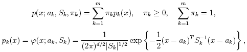
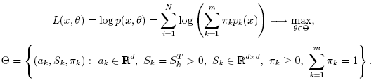
Consider the set of the feature vectors {x1, x2,..., xN}:
N vectors from d-dimensional Euclidean space drawn from a Gaussian mixture:
m is the number of mixtures, pk
is the normal distribution density with the mean ak
and covariance matrix Sk, πk is the weight of k-th mixture.
Given the number of mixtures m and the samples {xi, i=1..N}
the algorithm finds the maximum-likelihood estimates (MLE)
of the all the mixture parameters, i.e. ak, Sk and
πk:
pi,k
(denoted αi,k in the formula below)
of sample #i to belong to mixture #k
using the currently available mixture parameter estimates:
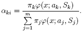
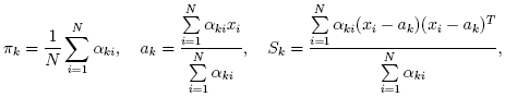
pi,k
can be provided. Another alternative, when pi,k are unknown,
is to use a simpler clustering algorithm to pre-cluster the input samples and thus obtain
initial pi,k. Often (and in ML)
k-means algorithm is used for that purpose.
One of the main that EM algorithm should deal with is the large number of parameters to estimate.
The majority of the parameters sits in covariation matrices, which are d×d elements each
(where d is the feature space dimensionality). However, in many practical problems
the covariation matrices are close to diagonal, or even to μk*I,
where I is identity matrix and μk is mixture-dependent "scale" parameter.
So a robust computation scheme could be to start with the harder constraints on
the covariation matrices and then use the estimated parameters as an input for
a less constrained optimization problem (often a diagonal covariation matrix is already a good enough
approximation).
References:
Parameters of EM algorithm
struct CvEMParams
{
    CvEMParams() : nclusters(10), cov_mat_type(CvEM::COV_MAT_DIAGONAL),
        start_step(CvEM::START_AUTO_STEP), probs(0), weights(0), means(0), covs(0)
    {
        term_crit=cvTermCriteria( CV_TERMCRIT_ITER+CV_TERMCRIT_EPS, 100, FLT_EPSILON );
    }

    CvEMParams( int _nclusters, int _cov_mat_type=1/*CvEM::COV_MAT_DIAGONAL*/,
                int _start_step=0/*CvEM::START_AUTO_STEP*/,
                CvTermCriteria _term_crit=cvTermCriteria(CV_TERMCRIT_ITER+CV_TERMCRIT_EPS, 100, FLT_EPSILON),
                CvMat* _probs=0, CvMat* _weights=0, CvMat* _means=0, CvMat** _covs=0 ) :
                nclusters(_nclusters), cov_mat_type(_cov_mat_type), start_step(_start_step),
                probs(_probs), weights(_weights), means(_means), covs(_covs), term_crit(_term_crit)
    {}

    int nclusters;
    int cov_mat_type;
    int start_step;
    const CvMat* probs;
    const CvMat* weights;
    const CvMat* means;
    const CvMat** covs;
    CvTermCriteria term_crit;
};
CvEM::COV_MAT_GENERIC - a covariation matrix of each mixture may
be arbitrary symmetrical positively defined matrix,
so the number of free parameters in each matrix
is about d2/2. It is not recommended to use this option,
unless there is pretty accurate initial estimation of the parameters and/or
a huge number of training samples.CvEM::COV_MAT_DIAGONAL - a covariation matrix of each mixture may
be arbitrary diagonal matrix with positive diagonal elements, that is, non-diagonal
elements are forced to be 0's, so the number of free parameters is d
for each matrix. This is most commonly used option yielding good estimation results.CvEM::COV_MAT_SPHERICAL - a covariation matrix of each mixture is a scaled
identity matrix, μk*I, so the only parameter to be
estimated is μk. The option may be used in special cases,
when the constraint is relevant, or as a first step in the optimization (e.g.
in case when the data is preprocessed with
PCA).
The results of such preliminary estimation may be passed again to the optimization
procedure, this time with cov_mat_type=CvEM::COV_MAT_DIAGONAL.
CvEM::START_E_STEP - the algorithm starts with E-step. At least,
the initial values of mean vectors, CvEMParams::means must be
passed. Optionally, the user may also provide initial values for weights
(CvEMParams::weights) and/or covariation matrices
(CvEMParams::covs).CvEM::START_M_STEP - the algorithm starts with M-step.
The initial probabilities pi,k must be provided.CvEM::START_AUTO_STEP - No values are required from
the user,
k-means algorithm is used to estimate initial mixtures parameters.
term_crit.num_iter),
or when the parameters change too little (no more than term_crit.epsilon)
from iteration to iteration.
pi,k; are used (and must be not NULL) only when start_step=CvEM::START_M_STEP.
πk; are used (if not NULL) only when start_step=CvEM::START_E_STEP.
Sk; are used (if not NULL) only when start_step=CvEM::START_E_STEP.
ak; are used (and must be not NULL) only when start_step=CvEM::START_E_STEP.
The structure has 2 constructors, the default one represents a rough rule-of-thumb, with another one it is possible to override a variety of parameters, from a single number of mixtures (the only essential problem-dependent parameter), to the initial values for the mixture parameters.
EM model
class CV_EXPORTS CvEM : public CvStatModel
{
public:
    // Type of covariation matrices
    enum { COV_MAT_SPHERICAL=0, COV_MAT_DIAGONAL=1, COV_MAT_GENERIC=2 };

    // The initial step
    enum { START_E_STEP=1, START_M_STEP=2, START_AUTO_STEP=0 };

    CvEM();
    CvEM( const CvMat* samples, const CvMat* sample_idx=0,
          CvEMParams params=CvEMParams(), CvMat* labels=0 );
    virtual ~CvEM();

    virtual bool train( const CvMat* samples, const CvMat* sample_idx=0,
                        CvEMParams params=CvEMParams(), CvMat* labels=0 );

    virtual float predict( const CvMat* sample, CvMat* probs ) const;
    virtual void clear();

    int get_nclusters() const { return params.nclusters; }
    const CvMat* get_means() const { return means; }
    const CvMat** get_covs() const { return covs; }
    const CvMat* get_weights() const { return weights; }
    const CvMat* get_probs() const { return probs; }

protected:

    virtual void set_params( const CvEMParams& params,
                             const CvVectors& train_data );
    virtual void init_em( const CvVectors& train_data );
    virtual double run_em( const CvVectors& train_data );
    virtual void init_auto( const CvVectors& samples );
    virtual void kmeans( const CvVectors& train_data, int nclusters,
                         CvMat* labels, CvTermCriteria criteria,
                         const CvMat* means );
    CvEMParams params;
    double log_likelihood;

    CvMat* means;
    CvMat** covs;
    CvMat* weights;
    CvMat* probs;

    CvMat* log_weight_div_det;
    CvMat* inv_eigen_values;
    CvMat** cov_rotate_mats;
};
Estimates Gaussian mixture parameters from the sample set
void CvEM::train( const CvMat* samples, const CvMat*  sample_idx=0,
                  CvEMParams params=CvEMParams(), CvMat* labels=0 );
Unlike many of ML models, EM is an unsupervised learning algorithm and it does not
take responses (class labels or the function values) on input. Instead, it computes
MLE of Gaussian mixture parameters from the input sample set,
stores all the parameters inside the stucture: pi,k in probs,
ak in means Sk in covs[k],
πk in weights and
optionally computes the output "class label" for each sample:
labelsi=arg maxk(pi,k), i=1..N
(i.e. indices of the most-probable mixture for each sample).
The trained model can be used further for prediction, just like any other classifier. The model trained is similar to the normal bayes classifier.
#include "ml.h"
#include "highgui.h"

int main( int argc, char** argv )
{
    const int N = 4;
    const int N1 = (int)sqrt((double)N);
    const CvScalar colors[] = {{{0,0,255}},{{0,255,0}},{{0,255,255}},{{255,255,0}}};
    int i, j;
    int nsamples = 100;
    CvRNG rng_state = cvRNG(-1);
    CvMat* samples = cvCreateMat( nsamples, 2, CV_32FC1 );
    CvMat* labels = cvCreateMat( nsamples, 1, CV_32SC1 );
    IplImage* img = cvCreateImage( cvSize( 500, 500 ), 8, 3 );
    float _sample[2];
    CvMat sample = cvMat( 1, 2, CV_32FC1, _sample );
    CvEM em_model;
    CvEMParams params;
    CvMat samples_part;

    cvReshape( samples, samples, 2, 0 );
    for( i = 0; i < N; i++ )
    {
        CvScalar mean, sigma;

        // form the training samples
        cvGetRows( samples, &samples_part, i*nsamples/N, (i+1)*nsamples/N );
        mean = cvScalar(((i%N1)+1.)*img->width/(N1+1), ((i/N1)+1.)*img->height/(N1+1));
        sigma = cvScalar(30,30);
        cvRandArr( &rng_state, &samples_part, CV_RAND_NORMAL, mean, sigma );
    }
    cvReshape( samples, samples, 1, 0 );

    // initialize model's parameters
    params.covs      = NULL;
    params.means     = NULL;
    params.weights   = NULL;
    params.probs     = NULL;
    params.nclusters = N;
    params.cov_mat_type       = CvEM::COV_MAT_SPHERICAL;
    params.start_step         = CvEM::START_AUTO_STEP;
    params.term_crit.max_iter = 10;
    params.term_crit.epsilon  = 0.1;
    params.term_crit.type     = CV_TERMCRIT_ITER|CV_TERMCRIT_EPS;

    // cluster the data
    em_model.train( samples, 0, params, labels );

#if 0
    // the piece of code shows how to repeatedly optimize the model
    // with less-constrained parameters (COV_MAT_DIAGONAL instead of COV_MAT_SPHERICAL)
    // when the output of the first stage is used as input for the second.
    CvEM em_model2;
    params.cov_mat_type = CvEM::COV_MAT_DIAGONAL;
    params.start_step = CvEM::START_E_STEP;
    params.means = em_model.get_means();
    params.covs = (const CvMat**)em_model.get_covs();
    params.weights = em_model.get_weights();

    em_model2.train( samples, 0, params, labels );
    // to use em_model2, replace em_model.predict() with em_model2.predict() below
#endif
    // classify every image pixel
    cvZero( img );
    for( i = 0; i < img->height; i++ )
    {
        for( j = 0; j < img->width; j++ )
        {
            CvPoint pt = cvPoint(j, i);
            sample.data.fl[0] = (float)j;
            sample.data.fl[1] = (float)i;
            int response = cvRound(em_model.predict( &sample, NULL ));
            CvScalar c = colors[response];

            cvCircle( img, pt, 1, cvScalar(c.val[0]*0.75,c.val[1]*0.75,c.val[2]*0.75), CV_FILLED );
        }
    }

    //draw the clustered samples
    for( i = 0; i < nsamples; i++ )
    {
        CvPoint pt;
        pt.x = cvRound(samples->data.fl[i*2]);
        pt.y = cvRound(samples->data.fl[i*2+1]);
        cvCircle( img, pt, 1, colors[labels->data.i[i]], CV_FILLED );
    }

    cvNamedWindow( "EM-clustering result", 1 );
    cvShowImage( "EM-clustering result", img );
    cvWaitKey(0);

    cvReleaseMat( &samples );
    cvReleaseMat( &labels );
    return 0;
}
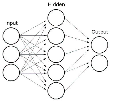
ML implements feedforward artificial neural networks, more particularly, multi-layer perceptrons (MLP), the most commonly used type of neural networks. MLP consists of the input layer, output layer and one or more hidden layers. Each layer of MLP includes one or more neurons that are directionally linked with the neurons from the previous and the next layer. Here is an example of 3-layer perceptron with 3 inputs, 2 outputs and the hidden layer including 5 neurons:
All the neurons in MLP are similar. Each of them has several input links (i.e.
it takes the output values from several neurons in the previous layer on input) and
several output links (i.e. it passes the response to several neurons in the next layer).
The values retrieved from the previous layer are summed with certain weights, individual for each
neuron, plus the bias term, and the sum is transformed using the activation function f that may be also
different for different neurons. Here is the picture:
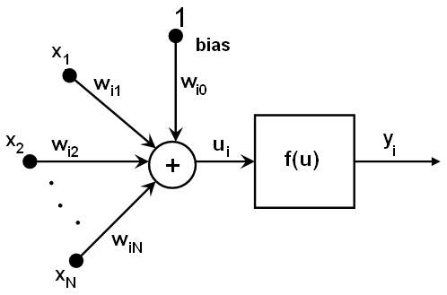
{xj} of the layer n,
the outputs {yi} of the layer n+1 are computed as:
    ui=sumj(w(n+1)i,j*xj) + w(n+1)i,bias
    yi=f(ui)
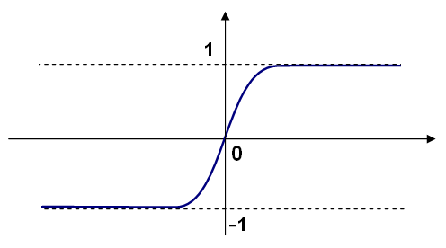
Different activation functions may be used, the ML implements 3 standard ones:
CvANN_MLP::IDENTITY): f(x)=x
CvANN_MLP::SIGMOID_SYM):
f(x)=β*(1-e-αx)/(1+e-αx),
the default choice for MLP; the standard sigmoid with β=1, α=1 is shown below:
CvANN_MLP::GAUSSIAN):
f(x)=βe-αx*x,
not completely supported by the moment.
In ML all the neurons have the same activation functions, with the same free parameters (α, β) that are specified by user and are not altered by the training algorithms.
So the whole trained network works as following. It takes the feature vector on input, the vector size is equal to the size of the input layer, when the values are passed as input to the first hidden layer, the outputs of the hidden layer are computed using the weights and the activation functions and passed further downstream, until we compute the output layer.
So, in order to compute the network one need to know all the weights w(n+1)i,j.
The weights are computed by the training algorithm. The algorithm takes a training set: multiple
input vectors with the corresponding output vectors, and iteratively adjusts the weights to try to make
the network give the desired response on the provided input vectors.
The larger the network size (the number of hidden layers and their sizes), the more is the potential network flexibility, and the error on the training set could be made arbitrarily small. But at the same time the learned network will also "learn" the noise present in the training set, so the error on the test set usually starts increasing after the network size reaches some limit. Besides, the larger networks are train much longer than the smaller ones, so it is reasonable to preprocess the data (using PCA or similar technique) and train a smaller network on only the essential features.
Another feature of the MLP's is their inability to handle categorical data as is, however
there is a workaround. If a certain
feature in the input or output (i.e. in case of n-class classifier for n>2)
layer is categorical and can take M (>2) different values,
it makes sense to represent it as binary tuple of M elements, where i-th
element is 1 if and only if the feature is equal to the i-th value out of
M possible. It will increase the size of the input/output layer, but will speedup the
training algorithm convergence and at the same time enable "fuzzy" values of such variables, i.e.
a tuple of probabilities instead of a fixed value.
ML implements 2 algorithms for training MLP's. The first is the classical random sequential backpropagation algorithm and the second (default one) is batch RPROP algorithm
References:
Parameters of MLP training algorithm
struct CvANN_MLP_TrainParams
{
    CvANN_MLP_TrainParams();
    CvANN_MLP_TrainParams( CvTermCriteria term_crit, int train_method,
                           double param1, double param2=0 );
    ~CvANN_MLP_TrainParams();

    enum { BACKPROP=0, RPROP=1 };

    CvTermCriteria term_crit;
    int train_method;

    // backpropagation parameters
    double bp_dw_scale, bp_moment_scale;

    // rprop parameters
    double rp_dw0, rp_dw_plus, rp_dw_minus, rp_dw_min, rp_dw_max;
};
CvANN_MLP_TrainParams::BACKPROP (sequential
backpropagation algorithm) or CvANN_MLP_TrainParams::RPROP
(RPROP algorithm, default value).
0.1. The parameter
can be set via param1 of the constructor.
0 (the feature is disabled)
to 1 and beyond. The value 0.1 or so is good enough.
The parameter can be set via param2 of the constructor.
0.1.
This parameter can be set via param1 of the constructor.
1.2 that should work well in most cases, according to
the algorithm's author. The parameter can only be changed explicitly by modifying the structure member.
0.5 that should work well in most cases, according to
the algorithm's author. The parameter can only be changed explicitly by modifying the structure member.
FLT_EPSILON.
The parameter can be set via param2 of the constructor.
50.
The parameter can only be changed explicitly by modifying the structure member.
The structure has default constructor that initializes parameters for RPROP algorithm.
There is also more advanced constructor to customize the parameters and/or choose backpropagation algorithm.
Finally, the individual parameters can be adjusted after the structure is created.
MLP model
class CvANN_MLP : public CvStatModel
{
public:
    CvANN_MLP();
    CvANN_MLP( const CvMat* _layer_sizes,
               int _activ_func=SIGMOID_SYM,
               double _f_param1=0, double _f_param2=0 );

    virtual ~CvANN_MLP();

    virtual void create( const CvMat* _layer_sizes,
                         int _activ_func=SIGMOID_SYM,
                         double _f_param1=0, double _f_param2=0 );

    virtual int train( const CvMat* _inputs, const CvMat* _outputs,
                       const CvMat* _sample_weights, const CvMat* _sample_idx=0,
                       CvANN_MLP_TrainParams _params = CvANN_MLP_TrainParams(),
                       int flags=0 );
    virtual float predict( const CvMat* _inputs,
                           CvMat* _outputs ) const;

    virtual void clear();

    // possible activation functions
    enum { IDENTITY = 0, SIGMOID_SYM = 1, GAUSSIAN = 2 };

    // available training flags
    enum { UPDATE_WEIGHTS = 1, NO_INPUT_SCALE = 2, NO_OUTPUT_SCALE = 4 };

    virtual void read( CvFileStorage* fs, CvFileNode* node );
    virtual void write( CvFileStorage* storage, const char* name );

    int get_layer_count() { return layer_sizes ? layer_sizes->cols : 0; }
    const CvMat* get_layer_sizes() { return layer_sizes; }

protected:

    virtual bool prepare_to_train( const CvMat* _inputs, const CvMat* _outputs,
            const CvMat* _sample_weights, const CvMat* _sample_idx,
            CvANN_MLP_TrainParams _params,
            CvVectors* _ivecs, CvVectors* _ovecs, double** _sw, int _flags );

    // sequential random backpropagation
    virtual int train_backprop( CvVectors _ivecs, CvVectors _ovecs, const double* _sw );

    // RPROP algorithm
    virtual int train_rprop( CvVectors _ivecs, CvVectors _ovecs, const double* _sw );

    virtual void calc_activ_func( CvMat* xf, const double* bias ) const;
    virtual void calc_activ_func_deriv( CvMat* xf, CvMat* deriv, const double* bias ) const;
    virtual void set_activ_func( int _activ_func=SIGMOID_SYM,
                                 double _f_param1=0, double _f_param2=0 );
    virtual void init_weights();
    virtual void scale_input( const CvMat* _src, CvMat* _dst ) const;
    virtual void scale_output( const CvMat* _src, CvMat* _dst ) const;
    virtual void calc_input_scale( const CvVectors* vecs, int flags );
    virtual void calc_output_scale( const CvVectors* vecs, int flags );

    virtual void write_params( CvFileStorage* fs );
    virtual void read_params( CvFileStorage* fs, CvFileNode* node );

    CvMat* layer_sizes;
    CvMat* wbuf;
    CvMat* sample_weights;
    double** weights;
    double f_param1, f_param2;
    double min_val, max_val, min_val1, max_val1;
    int activ_func;
    int max_count, max_buf_sz;
    CvANN_MLP_TrainParams params;
    CvRNG rng;
};
Unlike many other models in ML that are constructed and trained at once, in the MLP model these steps are separated. First, a network with the specified topology is created using the non-default constructor or the method create. All the weights are set to zeros. Then the network is trained using the set of input and output vectors. The training procedure can be repeated more than once, i.e. the weights can be adjusted based on the new training data.
Constructs the MLP with the specified topology
void CvANN_MLP::create( const CvMat* _layer_sizes,
                        int _activ_func=SIGMOID_SYM,
                        double _f_param1=0, double _f_param2=0 );
CvANN_MLP::IDENTITY, CvANN_MLP::SIGMOID_SYM
and CvANN_MLP::GAUSSIAN.
The method creates MLP network with the specified topology and assigns the same activation function to all the neurons.
Trains/updates MLP
int CvANN_MLP::train( const CvMat* _inputs, const CvMat* _outputs,
                      const CvMat* _sample_weights, const CvMat* _sample_idx=0,
                      CvANN_MLP_TrainParams _params = CvANN_MLP_TrainParams(),
                      int flags=0 );
_inputs and _outputs) that are taken
into account.
UPDATE_WEIGHTS = 1 - algorithm updates the network weights, rather than
computes them from scratch (in the latter case the weights are
initialized
using Nguyen-Widrow algorithm).NO_INPUT_SCALE - algorithm does not normalize the input vectors. If this flag is not set,
the training algorithm normalizes each input feature independently, shifting its
mean value to 0 and making the standard deviation =1. If the network
is assumed to be updated frequently, the new training data could be much different from
original one. In this case user should take care of proper normalization.NO_OUTPUT_SCALE - algorithm does not normalize the output vectors. If the flag is not set,
the training algorithm normalizes each output features independently, by
transforming
it to the certain range depending on the activation function used.This method applies the specified training algorithm to compute/adjust the network weights. It returns the number of done iterations.