Motion Analysis and Object Tracking
Acc
- Acc(image, sum, mask=NULL) → None
Adds a frame to an accumulator.
Parameters:
The function adds the whole image image or its selected region to the accumulator sum :

CalcGlobalOrientation
- CalcGlobalOrientation(orientation, mask, mhi, timestamp, duration) → float
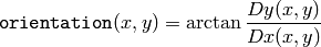
Calculates the global motion orientation of some selected region.
Parameters: - orientation (CvArr) – Motion gradient orientation image; calculated by the function CalcMotionGradient
- mask (CvArr) – Mask image. It may be a conjunction of a valid gradient mask, obtained with CalcMotionGradient and the mask of the region, whose direction needs to be calculated
- mhi (CvArr) – Motion history image
- timestamp (float) – Current time in milliseconds or other units, it is better to store time passed to UpdateMotionHistory before and reuse it here, because running UpdateMotionHistory and CalcMotionGradient on large images may take some time
- duration (float) – Maximal duration of motion track in milliseconds, the same as UpdateMotionHistory
The function calculates the general motion direction in the selected region and returns the angle between 0 degrees and 360 degrees . At first the function builds the orientation histogram and finds the basic orientation as a coordinate of the histogram maximum. After that the function calculates the shift relative to the basic orientation as a weighted sum of all of the orientation vectors: the more recent the motion, the greater the weight. The resultant angle is a circular sum of the basic orientation and the shift.
CalcMotionGradient
- CalcMotionGradient(mhi, mask, orientation, delta1, delta2, apertureSize=3) → None
Calculates the gradient orientation of a motion history image.
Parameters: - mhi (CvArr) – Motion history image
- mask (CvArr) – Mask image; marks pixels where the motion gradient data is correct; output parameter
- orientation (CvArr) – Motion gradient orientation image; contains angles from 0 to ~360 degrees
- delta1 (float) – See below
- delta2 (float) – See below
- apertureSize (int) – Aperture size of derivative operators used by the function: CV _ SCHARR, 1, 3, 5 or 7 (see Sobel )
The function calculates the derivatives
 and
and
 of
mhi
and then calculates gradient orientation as:
of
mhi
and then calculates gradient orientation as:
where both
 and
and
 signs are taken into account (as in the
CartToPolar
function). After that
mask
is filled to indicate where the orientation is valid (see the
delta1
and
delta2
description).
signs are taken into account (as in the
CartToPolar
function). After that
mask
is filled to indicate where the orientation is valid (see the
delta1
and
delta2
description).
The function finds the minimum (
 ) and maximum (
 ) mhi values over each pixel
 neighborhood and assumes the gradient is valid only if

CalcOpticalFlowBM
- CalcOpticalFlowBM(prev, curr, blockSize, shiftSize, max_range, usePrevious, velx, vely) → None
Calculates the optical flow for two images by using the block matching method.
Parameters: - prev (CvArr) – First image, 8-bit, single-channel
- curr (CvArr) – Second image, 8-bit, single-channel
- blockSize (CvSize) – Size of basic blocks that are compared
- shiftSize (CvSize) – Block coordinate increments
- max_range (CvSize) – Size of the scanned neighborhood in pixels around the block
- usePrevious (int) – Uses the previous (input) velocity field
- velx (CvArr) –
Horizontal component of the optical flow of

size, 32-bit floating-point, single-channel
- vely (CvArr) – Vertical component of the optical flow of the same size velx , 32-bit floating-point, single-channel
The function calculates the optical
flow for overlapped blocks
 pixels each, thus the velocity
fields are smaller than the original images. For every block in
prev
the functions tries to find a similar block in
curr
in some neighborhood of the original block or shifted by (velx(x0,y0),vely(x0,y0)) block as has been calculated by previous
function call (if
usePrevious=1
)
pixels each, thus the velocity
fields are smaller than the original images. For every block in
prev
the functions tries to find a similar block in
curr
in some neighborhood of the original block or shifted by (velx(x0,y0),vely(x0,y0)) block as has been calculated by previous
function call (if
usePrevious=1
)
CalcOpticalFlowHS
- CalcOpticalFlowHS(prev, curr, usePrevious, velx, vely, lambda, criteria) → None
Calculates the optical flow for two images.
Parameters: - prev (CvArr) – First image, 8-bit, single-channel
- curr (CvArr) – Second image, 8-bit, single-channel
- usePrevious (int) – Uses the previous (input) velocity field
- velx (CvArr) – Horizontal component of the optical flow of the same size as input images, 32-bit floating-point, single-channel
- vely (CvArr) – Vertical component of the optical flow of the same size as input images, 32-bit floating-point, single-channel
- lambda (float) – Lagrangian multiplier
- criteria (CvTermCriteria) – Criteria of termination of velocity computing
The function computes the flow for every pixel of the first input image using the Horn and Schunck algorithm [Horn81] .
CalcOpticalFlowLK
- CalcOpticalFlowLK(prev, curr, winSize, velx, vely) → None
Calculates the optical flow for two images.
Parameters: - prev (CvArr) – First image, 8-bit, single-channel
- curr (CvArr) – Second image, 8-bit, single-channel
- winSize (CvSize) – Size of the averaging window used for grouping pixels
- velx (CvArr) – Horizontal component of the optical flow of the same size as input images, 32-bit floating-point, single-channel
- vely (CvArr) – Vertical component of the optical flow of the same size as input images, 32-bit floating-point, single-channel
The function computes the flow for every pixel of the first input image using the Lucas and Kanade algorithm [Lucas81] .
CalcOpticalFlowPyrLK
CalcOpticalFlowPyrLK( prev, curr, prevPyr, currPyr, prevFeatures, winSize, level, criteria, flags, guesses = None) -> (currFeatures, status, track_error)
Calculates the optical flow for a sparse feature set using the iterative Lucas-Kanade method with pyramids.
param prev: First frame, at time t
type prev: param curr: Second frame, at time t + dt
type curr: param prevPyr: Buffer for the pyramid for the first frame. If the pointer is not NULL , the buffer must have a sufficient size to store the pyramid from level 1 to level level ; the total size of (image_width+8)*image_height/3 bytes is sufficient
type prevPyr: param currPyr: Similar to prevPyr , used for the second frame
type currPyr: param prevFeatures: Array of points for which the flow needs to be found
type prevFeatures: param currFeatures: Array of 2D points containing the calculated new positions of the input features in the second image
type currFeatures: param winSize: Size of the search window of each pyramid level
type winSize: param level: Maximal pyramid level number. If 0 , pyramids are not used (single level), if 1 , two levels are used, etc
type level: int
param status: Array. Every element of the array is set to 1 if the flow for the corresponding feature has been found, 0 otherwise
type status: str
param track_error: Array of double numbers containing the difference between patches around the original and moved points. Optional parameter; can be NULL
type track_error: float
param criteria: Specifies when the iteration process of finding the flow for each point on each pyramid level should be stopped
type criteria: param flags: Miscellaneous flags:
- CV_LKFLOWPyr_A_READY pyramid for the first frame is precalculated before the call
- CV_LKFLOWPyr_B_READY pyramid for the second frame is precalculated before the call
type flags: int
param guesses: optional array of estimated coordinates of features in second frame, with same length as prevFeatures
type guesses:
The function implements the sparse iterative version of the Lucas-Kanade optical flow in pyramids [Bouguet00] . It calculates the coordinates of the feature points on the current video frame given their coordinates on the previous frame. The function finds the coordinates with sub-pixel accuracy.
Both parameters prevPyr and currPyr comply with the following rules: if the image pointer is 0, the function allocates the buffer internally, calculates the pyramid, and releases the buffer after processing. Otherwise, the function calculates the pyramid and stores it in the buffer unless the flag CV_LKFLOWPyr_A[B]_READY is set. The image should be large enough to fit the Gaussian pyramid data. After the function call both pyramids are calculated and the readiness flag for the corresponding image can be set in the next call (i.e., typically, for all the image pairs except the very first one CV_LKFLOWPyr_A_READY is set).
CamShift
- CamShift(prob_image, window, criteria)-> (int, comp, box)
Finds the object center, size, and orientation.
Parameters: - prob_image (CvArr) – Back projection of object histogram (see CalcBackProject )
- window (CvRect) – Initial search window
- criteria (CvTermCriteria) – Criteria applied to determine when the window search should be finished
- comp (CvConnectedComp) – Resultant structure that contains the converged search window coordinates ( comp->rect field) and the sum of all of the pixels inside the window ( comp->area field)
- box (CvBox2D) – Circumscribed box for the object.
The function implements the CAMSHIFT object tracking algrorithm [Bradski98] . First, it finds an object center using MeanShift and, after that, calculates the object size and orientation. The function returns number of iterations made within MeanShift .
The CamShiftTracker class declared in cv.hpp implements the color object tracker that uses the function.
CvKalman
- class CvKalman
Kalman filter state.
- MP
- number of measurement vector dimensions
- DP
- number of state vector dimensions
- CP
- number of control vector dimensions
- state_pre
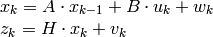
- predicted state (x’(k)): x(k)=A*x(k-1)+B*u(k)
- state_post
- corrected state (x(k)): x(k)=x’(k)+K(k)*(z(k)-H*x’(k))
- transition_matrix
- state transition matrix (A)
- control_matrix
- control matrix (B) (it is not used if there is no control)
- measurement_matrix
- measurement matrix (H)
- process_noise_cov
- process noise covariance matrix (Q)
- measurement_noise_cov
- measurement noise covariance matrix (R)
- error_cov_pre
- priori error estimate covariance matrix (P’(k)): P’(k)=A*P(k-1)*At + Q
- gain
- Kalman gain matrix (K(k)): K(k)=P’(k)*Ht*inv(H*P’(k)*Ht+R)
- error_cov_post
- posteriori error estimate covariance matrix (P(k)): P(k)=(I-K(k)*H)*P’(k)
The structure CvKalman is used to keep the Kalman filter state. It is created by the CreateKalman function, updated by the KalmanPredict and KalmanCorrect functions and released by the ReleaseKalman function. Normally, the structure is used for the standard Kalman filter (notation and the formulas below are borrowed from the excellent Kalman tutorial [Welch95] )
where:
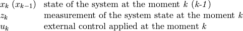
 and
and
 are normally-distributed process and measurement noise, respectively:
that is,
 process noise covariance matrix, constant or variable,
 measurement noise covariance matrix, constant or variable
In the case of the standard Kalman filter, all of the matrices: A, B, H, Q and R are initialized once after the CvKalman structure is allocated via CreateKalman . However, the same structure and the same functions may be used to simulate the extended Kalman filter by linearizing the extended Kalman filter equation in the current system state neighborhood, in this case A, B, H (and, probably, Q and R) should be updated on every step.
CreateKalman
CreateKalman(dynam_params, measure_params, control_params=0) -> CvKalman
Allocates the Kalman filter structure.
param dynam_params: dimensionality of the state vector type dynam_params: int param measure_params: dimensionality of the measurement vector type measure_params: int param control_params: dimensionality of the control vector type control_params: int
The function allocates CvKalman and all its matrices and initializes them somehow.
KalmanCorrect
KalmanCorrect(kalman, measurement) -> cvmat
Adjusts the model state.
param kalman: Kalman filter object returned by CreateKalman type kalman: CvKalman param measurement: CvMat containing the measurement vector type measurement: CvMat
The function adjusts the stochastic model state on the basis of the given measurement of the model state:
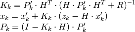
where
 |
given measurement ( mesurement parameter) |
|---|---|
 |
Kalman “gain” matrix. |
The function stores the adjusted state at kalman->state_post and returns it on output.
KalmanPredict
KalmanPredict(kalman, control=None) -> cvmat
Estimates the subsequent model state.
param kalman: Kalman filter object returned by CreateKalman type kalman: CvKalman param control: Control vector , should be NULL iff there is no external control ( control_params =0)
type control: CvMat
The function estimates the subsequent stochastic model state by its current state and stores it at kalman->state_pre :
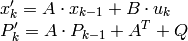
where
 |
is predicted state kalman->state_pre , |
|---|---|
 |
is corrected state on the previous step kalman->state_post (should be initialized somehow in the beginning, zero vector by default), |
|
is external control ( control parameter), |
 |
is priori error covariance matrix kalman->error_cov_pre |
 |
is posteriori error covariance matrix on the previous step kalman->error_cov_post (should be initialized somehow in the beginning, identity matrix by default), |
The function returns the estimated state.
KalmanUpdateByMeasurement
Synonym for KalmanCorrect
KalmanUpdateByTime
Synonym for KalmanPredict
MeanShift
- MeanShift(prob_image, window, criteria) → comp
Finds the object center on back projection.
Parameters: - prob_image (CvArr) – Back projection of the object histogram (see CalcBackProject )
- window (CvRect) – Initial search window
- criteria (CvTermCriteria) – Criteria applied to determine when the window search should be finished
- comp (CvConnectedComp) – Resultant structure that contains the converged search window coordinates ( comp->rect field) and the sum of all of the pixels inside the window ( comp->area field)
The function iterates to find the object center given its back projection and initial position of search window. The iterations are made until the search window center moves by less than the given value and/or until the function has done the maximum number of iterations. The function returns the number of iterations made.
MultiplyAcc
- MultiplyAcc(image1, image2, acc, mask=NULL) → None
Adds the product of two input images to the accumulator.
Parameters: - image1 (CvArr) – First input image, 1- or 3-channel, 8-bit or 32-bit floating point (each channel of multi-channel image is processed independently)
- image2 (CvArr) – Second input image, the same format as the first one
- acc (CvArr) – Accumulator with the same number of channels as input images, 32-bit or 64-bit floating-point
- mask (CvArr) – Optional operation mask
The function adds the product of 2 images or their selected regions to the accumulator acc :

RunningAvg
- RunningAvg(image, acc, alpha, mask=NULL) → None
Updates the running average.
Parameters: - image (CvArr) – Input image, 1- or 3-channel, 8-bit or 32-bit floating point (each channel of multi-channel image is processed independently)
- acc (CvArr) – Accumulator with the same number of channels as input image, 32-bit or 64-bit floating-point
- alpha (float) – Weight of input image
- mask (CvArr) – Optional operation mask
The function calculates the weighted sum of the input image image and the accumulator acc so that acc becomes a running average of frame sequence:

where
 regulates the update speed (how fast the accumulator forgets about previous frames).
SegmentMotion
- SegmentMotion(mhi, seg_mask, storage, timestamp, seg_thresh) → None
Segments a whole motion into separate moving parts.
Parameters: - mhi (CvArr) – Motion history image
- seg_mask (CvArr) – Image where the mask found should be stored, single-channel, 32-bit floating-point
- storage (CvMemStorage) – Memory storage that will contain a sequence of motion connected components
- timestamp (float) – Current time in milliseconds or other units
- seg_thresh (float) – Segmentation threshold; recommended to be equal to the interval between motion history “steps” or greater
The function finds all of the motion segments and marks them in seg_mask with individual values (1,2,...). It also returns a sequence of CvConnectedComp structures, one for each motion component. After that the motion direction for every component can be calculated with CalcGlobalOrientation using the extracted mask of the particular component Cmp .
SnakeImage
- SnakeImage(image, points, alpha, beta, gamma, coeff_usage, win, criteria, calc_gradient=1) → None
Changes the contour position to minimize its energy.
Parameters: - image (IplImage) – The source image or external energy field
- points (CvPoints) – Contour points (snake)
- alpha (sequence of int) – Weight[s] of continuity energy, single float or array of length floats, one for each contour point
- beta (sequence of int) – Weight[s] of curvature energy, similar to alpha
- gamma (sequence of int) – Weight[s] of image energy, similar to alpha
- coeff_usage (int) –
Different uses of the previous three parameters:
- CV_VALUE indicates that each of alpha, beta, gamma is a pointer to a single value to be used for all points;
- CV_ARRAY indicates that each of alpha, beta, gamma is a pointer to an array of coefficients different for all the points of the snake. All the arrays must have the size equal to the contour size.
- win (CvSize) – Size of neighborhood of every point used to search the minimum, both win.width and win.height must be odd
- criteria (CvTermCriteria) – Termination criteria
- calc_gradient (int) – Gradient flag; if not 0, the function calculates the gradient magnitude for every image pixel and consideres it as the energy field, otherwise the input image itself is considered
The function updates the snake in order to minimize its total energy that is a sum of internal energy that depends on the contour shape (the smoother contour is, the smaller internal energy is) and external energy that depends on the energy field and reaches minimum at the local energy extremums that correspond to the image edges in the case of using an image gradient.
The parameter criteria.epsilon is used to define the minimal number of points that must be moved during any iteration to keep the iteration process running.
If at some iteration the number of moved points is less than criteria.epsilon or the function performed criteria.max_iter iterations, the function terminates.
SquareAcc
- SquareAcc(image, sqsum, mask=NULL) → None
Adds the square of the source image to the accumulator.
Parameters:
The function adds the input image image or its selected region, raised to power 2, to the accumulator sqsum :

UpdateMotionHistory
- UpdateMotionHistory(silhouette, mhi, timestamp, duration) → None
Updates the motion history image by a moving silhouette.
Parameters: - silhouette (CvArr) – Silhouette mask that has non-zero pixels where the motion occurs
- mhi (CvArr) – Motion history image, that is updated by the function (single-channel, 32-bit floating-point)
- timestamp (float) – Current time in milliseconds or other units
- duration (float) – Maximal duration of the motion track in the same units as timestamp
The function updates the motion history image as following:

That is, MHI pixels where motion occurs are set to the current timestamp, while the pixels where motion happened far ago are cleared.
Help and Feedback
You did not find what you were looking for?- Try the FAQ.
- Ask a question in the user group/mailing list.
- If you think something is missing or wrong in the documentation, please file a bug report.
![]()
Table Of Contents
- Motion Analysis and Object Tracking
- Acc
- CalcGlobalOrientation
- CalcMotionGradient
- CalcOpticalFlowBM
- CalcOpticalFlowHS
- CalcOpticalFlowLK
- CalcOpticalFlowPyrLK
- CamShift
- CvKalman
- CreateKalman
- KalmanCorrect
- KalmanPredict
- KalmanUpdateByMeasurement
- KalmanUpdateByTime
- MeanShift
- MultiplyAcc
- RunningAvg
- SegmentMotion
- SnakeImage
- SquareAcc
- UpdateMotionHistory
Previous topic
Next topic
Structural Analysis and Shape Descriptors