Operations on Arrays
cv::abs
- MatExpr<...> abs(const MatExpr<...>& src)
Computes absolute value of each matrix element
Parameters: - src – matrix or matrix expression
abs is a meta-function that is expanded to one of absdiff() forms:
- C = abs(A-B) is equivalent to absdiff(A, B, C) and
- C = abs(A) is equivalent to absdiff(A, Scalar::all(0), C) .
- C = Mat_<Vec<uchar,n> >(abs(A*alpha + beta)) is equivalent to convertScaleAbs(A, C, alpha, beta)
The output matrix will have the same size and the same type as the input one (except for the last case, where C will be depth=CV_8U ).
See also: Matrix Expressions , absdiff() ,
cv::absdiff
- void absdiff(const MatND& src1, const MatND& src2, MatND& dst)
- void absdiff(const MatND& src1, const Scalar& sc, MatND& dst)
Computes per-element absolute difference between 2 arrays or between array and a scalar.
Parameters: - src1 – The first input array
- src2 – The second input array; Must be the same size and same type as src1
- sc – Scalar; the second input parameter
- dst – The destination array; it will have the same size and same type as src1 ; see Mat::create
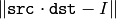
The functions absdiff compute:
absolute difference between two arrays

or absolute difference between array and a scalar:

where I is multi-dimensional index of array elements. in the case of multi-channel arrays each channel is processed independently.
See also: abs() ,
cv::add
- void add(const MatND& src1, const MatND& src2, MatND& dst)
- void add(const MatND& src1, const MatND& src2, MatND& dst, const MatND& mask)
- void add(const MatND& src1, const Scalar& sc, MatND& dst, const MatND& mask=MatND())
Computes the per-element sum of two arrays or an array and a scalar.
Parameters: - src1 – The first source array
- src2 – The second source array. It must have the same size and same type as src1
- sc – Scalar; the second input parameter
- dst – The destination array; it will have the same size and same type as src1 ; see Mat::create
- mask – The optional operation mask, 8-bit single channel array; specifies elements of the destination array to be changed
The functions add compute:
the sum of two arrays:

or the sum of array and a scalar:

where I is multi-dimensional index of array elements.
The first function in the above list can be replaced with matrix expressions:
dst = src1 + src2;
dst += src1; // equivalent to add(dst, src1, dst);
in the case of multi-channel arrays each channel is processed independently.
See also: subtract() , addWeighted() , scaleAdd() , convertScale() , Matrix Expressions , .
cv::addWeighted
- void addWeighted(const Mat& src1, double alpha, const Mat& src2, double beta, double gamma, Mat& dst)
- void addWeighted(const MatND& src1, double alpha, const MatND& src2, double beta, double gamma, MatND& dst)
Computes the weighted sum of two arrays.
Parameters: - src1 – The first source array
- alpha – Weight for the first array elements
- src2 – The second source array; must have the same size and same type as src1
- beta – Weight for the second array elements
- dst – The destination array; it will have the same size and same type as src1
- gamma – Scalar, added to each sum
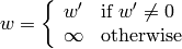
The functions addWeighted calculate the weighted sum of two arrays as follows:

where I is multi-dimensional index of array elements.
The first function can be replaced with a matrix expression:
dst = src1*alpha + src2*beta + gamma;
In the case of multi-channel arrays each channel is processed independently.
See also: add() , subtract() , scaleAdd() , convertScale() , Matrix Expressions , .
bitwise_and
- void bitwise_and(const MatND& src1, const MatND& src2, MatND& dst, const MatND& mask=MatND())
- void bitwise_and(const MatND& src1, const Scalar& sc, MatND& dst, const MatND& mask=MatND())
Calculates per-element bit-wise conjunction of two arrays and an array and a scalar.
Parameters: - src1 – The first source array
- src2 – The second source array. It must have the same size and same type as src1
- sc – Scalar; the second input parameter
- dst – The destination array; it will have the same size and same type as src1 ; see Mat::create
- mask – The optional operation mask, 8-bit single channel array; specifies elements of the destination array to be changed
The functions bitwise_and compute per-element bit-wise logical conjunction:
of two arrays

or array and a scalar:

In the case of floating-point arrays their machine-specific bit representations (usually IEEE754-compliant) are used for the operation, and in the case of multi-channel arrays each channel is processed independently.
See also: , ,
bitwise_not
- void bitwise_not(const MatND& src, MatND& dst)
Inverts every bit of array
Parameters: - src1 – The source array
- dst – The destination array; it is reallocated to be of the same size and the same type as src ; see Mat::create
- mask – The optional operation mask, 8-bit single channel array; specifies elements of the destination array to be changed
The functions bitwise_not compute per-element bit-wise inversion of the source array:
In the case of floating-point source array its machine-specific bit representation (usually IEEE754-compliant) is used for the operation. in the case of multi-channel arrays each channel is processed independently.
See also: , ,
bitwise_or
- void bitwise_or(const MatND& src1, const MatND& src2, MatND& dst, const MatND& mask=MatND())
- void bitwise_or(const MatND& src1, const Scalar& sc, MatND& dst, const MatND& mask=MatND())
Calculates per-element bit-wise disjunction of two arrays and an array and a scalar.
Parameters: - src1 – The first source array
- src2 – The second source array. It must have the same size and same type as src1
- sc – Scalar; the second input parameter
- dst – The destination array; it is reallocated to be of the same size and the same type as src1 ; see Mat::create
- mask – The optional operation mask, 8-bit single channel array; specifies elements of the destination array to be changed
The functions bitwise_or compute per-element bit-wise logical disjunction
of two arrays

or array and a scalar:

In the case of floating-point arrays their machine-specific bit representations (usually IEEE754-compliant) are used for the operation. in the case of multi-channel arrays each channel is processed independently.
See also: , ,
bitwise_xor
- void bitwise_xor(const MatND& src1, const MatND& src2, MatND& dst, const MatND& mask=MatND())
- void bitwise_xor(const MatND& src1, const Scalar& sc, MatND& dst, const MatND& mask=MatND())
Calculates per-element bit-wise “exclusive or” operation on two arrays and an array and a scalar.
Parameters: - src1 – The first source array
- src2 – The second source array. It must have the same size and same type as src1
- sc – Scalar; the second input parameter
- dst – The destination array; it is reallocated to be of the same size and the same type as src1 ; see Mat::create
- mask – The optional operation mask, 8-bit single channel array; specifies elements of the destination array to be changed
The functions bitwise_xor compute per-element bit-wise logical “exclusive or” operation
on two arrays

or array and a scalar:

In the case of floating-point arrays their machine-specific bit representations (usually IEEE754-compliant) are used for the operation. in the case of multi-channel arrays each channel is processed independently.
See also: , ,
cv::calcCovarMatrix
- void calcCovarMatrix(const Mat* samples, int nsamples, Mat& covar, Mat& mean, int flags, int ctype=CV_64F)
- void calcCovarMatrix(const Mat& samples, Mat& covar, Mat& mean, int flags, int ctype=CV_64F)
Calculates covariation matrix of a set of vectors
Parameters: - samples – The samples, stored as separate matrices, or as rows or columns of a single matrix
- nsamples – The number of samples when they are stored separately
- covar – The output covariance matrix; it will have type= ctype and square size
- mean – The input or output (depending on the flags) array - the mean (average) vector of the input vectors
- flags –
The operation flags, a combination of the following values
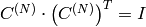
- CV_COVAR_SCRAMBLED The output covariance matrix is calculated as:
![\texttt{scale} \cdot [ \texttt{vects} [0]- \texttt{mean} , \texttt{vects} [1]- \texttt{mean} ,...]^T \cdot [ \texttt{vects} [0]- \texttt{mean} , \texttt{vects} [1]- \texttt{mean} ,...]](_images/math/131c7329c69299d33cd4cc9c62373a5885db9c5b.png)
, that is, the covariance matrix will be
 .
Such an unusual covariance matrix is used for fast PCA
of a set of very large vectors (see, for example, the EigenFaces technique
for face recognition). Eigenvalues of this “scrambled” matrix will
match the eigenvalues of the true covariance matrix and the “true”
eigenvectors can be easily calculated from the eigenvectors of the
“scrambled” covariance matrix.
.
Such an unusual covariance matrix is used for fast PCA
of a set of very large vectors (see, for example, the EigenFaces technique
for face recognition). Eigenvalues of this “scrambled” matrix will
match the eigenvalues of the true covariance matrix and the “true”
eigenvectors can be easily calculated from the eigenvectors of the
“scrambled” covariance matrix. - CV_COVAR_NORMAL The output covariance matrix is calculated as:
![\texttt{scale} \cdot [ \texttt{vects} [0]- \texttt{mean} , \texttt{vects} [1]- \texttt{mean} ,...] \cdot [ \texttt{vects} [0]- \texttt{mean} , \texttt{vects} [1]- \texttt{mean} ,...]^T](_images/math/8ea3c304dbd969d5def0866d587b87c5d96c6f58.png)
, that is, covar will be a square matrix of the same size as the total number of elements in each input vector. One and only one of CV_COVAR_SCRAMBLED and CV_COVAR_NORMAL must be specified
- CV_COVAR_USE_AVG If the flag is specified, the function does not calculate mean from the input vectors, but, instead, uses the passed mean vector. This is useful if mean has been pre-computed or known a-priori, or if the covariance matrix is calculated by parts - in this case, mean is not a mean vector of the input sub-set of vectors, but rather the mean vector of the whole set.
- CV_COVAR_SCALE If the flag is specified, the covariance matrix is scaled. In the “normal” mode scale is 1./nsamples ; in the “scrambled” mode scale is the reciprocal of the total number of elements in each input vector. By default (if the flag is not specified) the covariance matrix is not scaled (i.e. scale=1 ).
- CV_COVAR_ROWS [Only useful in the second variant of the function] The flag means that all the input vectors are stored as rows of the samples matrix. mean should be a single-row vector in this case.
- CV_COVAR_COLS [Only useful in the second variant of the function] The flag means that all the input vectors are stored as columns of the samples matrix. mean should be a single-column vector in this case.
- CV_COVAR_SCRAMBLED The output covariance matrix is calculated as:
The functions calcCovarMatrix calculate the covariance matrix and, optionally, the mean vector of the set of input vectors.
See also: PCA() , mulTransposed() , Mahalanobis()
cv::cartToPolar
- void cartToPolar(const Mat& x, const Mat& y, Mat& magnitude, Mat& angle, bool angleInDegrees=false)
Calculates the magnitude and angle of 2d vectors.
Parameters: - x – The array of x-coordinates; must be single-precision or double-precision floating-point array
- y – The array of y-coordinates; it must have the same size and same type as x
- magnitude – The destination array of magnitudes of the same size and same type as x
- angle – The destination array of angles of the same size and same type as x .
The angles are measured in radians
 to
to  or in degrees (0 to 360 degrees).
 - angleInDegrees – The flag indicating whether the angles are measured in radians, which is default mode, or in degrees
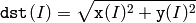
The function cartToPolar calculates either the magnitude, angle, or both of every 2d vector (x(I),y(I)):
![\begin{array}{l} \texttt{magnitude} (I)= \sqrt{\texttt{x}(I)^2+\texttt{y}(I)^2} , \\ \texttt{angle} (I)= \texttt{atan2} ( \texttt{y} (I), \texttt{x} (I))[ \cdot180 / \pi ] \end{array}](_images/math/bbfdf84dba415be8bfa0d6db434f1fd388cdcadb.png)
The angles are calculated with
 accuracy. For the (0,0) point, the angle is set to 0.
cv::checkRange
- bool checkRange(const Mat& src, bool quiet=true, Point* pos=0, double minVal=-DBL_MAX, double maxVal=DBL_MAX)
- bool checkRange(const MatND& src, bool quiet=true, int* pos=0, double minVal=-DBL_MAX, double maxVal=DBL_MAX)
Checks every element of an input array for invalid values.
Parameters: - src – The array to check
- quiet – The flag indicating whether the functions quietly return false when the array elements are out of range, or they throw an exception.
- pos – The optional output parameter, where the position of the first outlier is stored. In the second function pos , when not NULL, must be a pointer to array of src.dims elements
- minVal – The inclusive lower boundary of valid values range
- maxVal – The exclusive upper boundary of valid values range
The functions
checkRange
check that every array element is
neither NaN nor
 . When
minVal < -DBL_MAX
and
maxVal < DBL_MAX
, then the functions also check that
each value is between
minVal
and
maxVal
. in the case of multi-channel arrays each channel is processed independently.
If some values are out of range, position of the first outlier is stored in
pos
(when
. When
minVal < -DBL_MAX
and
maxVal < DBL_MAX
, then the functions also check that
each value is between
minVal
and
maxVal
. in the case of multi-channel arrays each channel is processed independently.
If some values are out of range, position of the first outlier is stored in
pos
(when
 ), and then the functions either return false (when
quiet=true
) or throw an exception.
), and then the functions either return false (when
quiet=true
) or throw an exception.
cv::compare
- void compare(const MatND& src1, const MatND& src2, MatND& dst, int cmpop)
- void compare(const MatND& src1, double value, MatND& dst, int cmpop)
Performs per-element comparison of two arrays or an array and scalar value.
Parameters: - src1 – The first source array
- src2 – The second source array; must have the same size and same type as src1
- value – The scalar value to compare each array element with
- dst – The destination array; will have the same size as src1 and type= CV_8UC1
- cmpop –
The flag specifying the relation between the elements to be checked
- CMP_EQ
 or
or 
- CMP_GT
 or
or 
- CMP_GE
 or
or 
- CMP_LT
 or
or 
- CMP_LE
 or
or 
- CMP_NE
 or
or 
- CMP_EQ
The functions compare compare each element of src1 with the corresponding element of src2 or with real scalar value . When the comparison result is true, the corresponding element of destination array is set to 255, otherwise it is set to 0:
- dst(I) = src1(I) cmpop src2(I) ? 255 : 0
- dst(I) = src1(I) cmpop value ? 255 : 0
The comparison operations can be replaced with the equivalent matrix expressions:
Mat dst1 = src1 >= src2;
Mat dst2 = src1 < 8;
...
See also: checkRange() , min() , max() , threshold() , Matrix Expressions
cv::completeSymm
- void completeSymm(Mat& mtx, bool lowerToUpper=false)
Copies the lower or the upper half of a square matrix to another half.
Parameters: - mtx – Input-output floating-point square matrix
- lowerToUpper – If true, the lower half is copied to the upper half, otherwise the upper half is copied to the lower half
The function completeSymm copies the lower half of a square matrix to its another half; the matrix diagonal remains unchanged:
 for
for
 if
lowerToUpper=false
if
lowerToUpper=false-
for
 if
lowerToUpper=true
if
lowerToUpper=true
See also: flip() , transpose()
cv::convertScaleAbs
- void convertScaleAbs(const Mat& src, Mat& dst, double alpha=1, double beta=0)
Scales, computes absolute values and converts the result to 8-bit.
Parameters: - src – The source array
- dst – The destination array
- alpha – The optional scale factor
- beta – The optional delta added to the scaled values
On each element of the input array the function convertScaleAbs performs 3 operations sequentially: scaling, taking absolute value, conversion to unsigned 8-bit type:

in the case of multi-channel arrays the function processes each channel independently. When the output is not 8-bit, the operation can be emulated by calling Mat::convertTo method (or by using matrix expressions) and then by computing absolute value of the result, for example:
Mat_<float> A(30,30);
randu(A, Scalar(-100), Scalar(100));
Mat_<float> B = A*5 + 3;
B = abs(B);
// Mat_<float> B = abs(A*5+3) will also do the job,
// but it will allocate a temporary matrix
See also: Mat::convertTo() , abs()
cv::countNonZero
- int countNonZero(const MatND& mtx)
Counts non-zero array elements.
Parameters: - mtx – Single-channel array
The function cvCountNonZero returns the number of non-zero elements in mtx:

See also: mean() , meanStdDev() , norm() , minMaxLoc() , calcCovarMatrix()
cv::cubeRoot
- float cubeRoot(float val)
Computes cube root of the argument
Parameters: - val – The function argument
The function
cubeRoot
computes
![\sqrt[3]{\texttt{val}}](_images/math/82540f5fd7cb0fee8d4e8fc93aeea6bb2b23054a.png) .
Negative arguments are handled correctly,
NaN
and
.
Negative arguments are handled correctly,
NaN
and
 are not handled.
The accuracy approaches the maximum possible accuracy for single-precision data.
are not handled.
The accuracy approaches the maximum possible accuracy for single-precision data.
cv::cvarrToMat
- Mat cvarrToMat(const CvArr* src, bool copyData=false, bool allowND=true, int coiMode=0)
Converts CvMat, IplImage or CvMatND to cv::Mat.
Parameters: - src – The source CvMat , IplImage or CvMatND
- copyData – When it is false (default value), no data is copied, only the new header is created. In this case the original array should not be deallocated while the new matrix header is used. The the parameter is true, all the data is copied, then user may deallocate the original array right after the conversion
- allowND – When it is true (default value), then CvMatND is converted to Mat if it’s possible (e.g. then the data is contiguous). If it’s not possible, or when the parameter is false, the function will report an error
- coiMode –
The parameter specifies how the IplImage COI (when set) is handled.
- If coiMode=0 , the function will report an error if COI is set.
- If coiMode=1 , the function will never report an error; instead it returns the header to the whole original image and user will have to check and process COI manually, see extractImageCOI() .
The function cvarrToMat converts CvMat , IplImage or CvMatND header to Mat() header, and optionally duplicates the underlying data. The constructed header is returned by the function.
When copyData=false , the conversion is done really fast (in O(1) time) and the newly created matrix header will have refcount=0 , which means that no reference counting is done for the matrix data, and user has to preserve the data until the new header is destructed. Otherwise, when copyData=true , the new buffer will be allocated and managed as if you created a new matrix from scratch and copy the data there. That is, cvarrToMat(src, true) :math:`\sim` cvarrToMat(src, false).clone() (assuming that COI is not set). The function provides uniform way of supporting CvArr paradigm in the code that is migrated to use new-style data structures internally. The reverse transformation, from Mat() to CvMat or IplImage can be done by simple assignment:
CvMat* A = cvCreateMat(10, 10, CV_32F);
cvSetIdentity(A);
IplImage A1; cvGetImage(A, &A1);
Mat B = cvarrToMat(A);
Mat B1 = cvarrToMat(&A1);
IplImage C = B;
CvMat C1 = B1;
// now A, A1, B, B1, C and C1 are different headers
// for the same 10x10 floating-point array.
// note, that you will need to use "&"
// to pass C & C1 to OpenCV functions, e.g:
printf("
Normally, the function is used to convert an old-style 2D array ( CvMat or IplImage ) to Mat , however, the function can also take CvMatND on input and create Mat() for it, if it’s possible. And for CvMatND A it is possible if and only if A.dim[i].size*A.dim.step[i] == A.dim.step[i-1] for all or for all but one i, 0 < i < A.dims . That is, the matrix data should be continuous or it should be representable as a sequence of continuous matrices. By using this function in this way, you can process CvMatND using arbitrary element-wise function. But for more complex operations, such as filtering functions, it will not work, and you need to convert CvMatND to MatND() using the corresponding constructor of the latter.
The last parameter, coiMode , specifies how to react on an image with COI set: by default it’s 0, and then the function reports an error when an image with COI comes in. And coiMode=1 means that no error is signaled - user has to check COI presence and handle it manually. The modern structures, such as Mat() and MatND() do not support COI natively. To process individual channel of an new-style array, you will need either to organize loop over the array (e.g. using matrix iterators) where the channel of interest will be processed, or extract the COI using mixChannels() (for new-style arrays) or extractImageCOI() (for old-style arrays), process this individual channel and insert it back to the destination array if need (using mixChannel() or insertImageCOI() , respectively).
See also: cvGetImage() , cvGetMat() , cvGetMatND() , extractImageCOI() , insertImageCOI() , mixChannels()
cv::dct
- void dct(const Mat& src, Mat& dst, int flags=0)
Performs a forward or inverse discrete cosine transform of 1D or 2D array
Parameters: - src – The source floating-point array
- dst – The destination array; will have the same size and same type as src
- flags –
Transformation flags, a combination of the following values
- DCT_INVERSE do an inverse 1D or 2D transform instead of the default forward transform.
- DCT_ROWS do a forward or inverse transform of every individual row of the input matrix. This flag allows user to transform multiple vectors simultaneously and can be used to decrease the overhead (which is sometimes several times larger than the processing itself), to do 3D and higher-dimensional transforms and so forth.
The function dct performs a forward or inverse discrete cosine transform (DCT) of a 1D or 2D floating-point array:
Forward Cosine transform of 1D vector of
 elements:
where
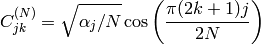
and
 ,
,
 for
for
 .
.
Inverse Cosine transform of 1D vector of N elements:
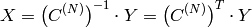
(since
 is orthogonal matrix,
 )
)
Forward Cosine transform of 2D
 matrix:
Inverse Cosine transform of 2D vector of
elements:
The function chooses the mode of operation by looking at the flags and size of the input array:
- if (flags & DCT_INVERSE) == 0 , the function does forward 1D or 2D transform, otherwise it is inverse 1D or 2D transform.
- if (flags & DCT_ROWS) :math:`\ne` 0 , the function performs 1D transform of each row.
- otherwise, if the array is a single column or a single row, the function performs 1D transform
- otherwise it performs 2D transform.
Important note : currently cv::dct supports even-size arrays (2, 4, 6 ...). For data analysis and approximation you can pad the array when necessary.
Also, the function’s performance depends very much, and not monotonically, on the array size, see
getOptimalDFTSize()
. In the current implementation DCT of a vector of size
N
is computed via DFT of a vector of size
N/2
, thus the optimal DCT size
 can be computed as:
size_t getOptimalDCTSize(size_t N) { return 2*getOptimalDFTSize((N+1)/2); }
See also: dft() , getOptimalDFTSize() , idct()
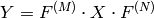
cv::dft
- void dft(const Mat& src, Mat& dst, int flags=0, int nonzeroRows=0)
Performs a forward or inverse Discrete Fourier transform of 1D or 2D floating-point array.
Parameters: - src – The source array, real or complex
- dst – The destination array, which size and type depends on the flags
- flags –
Transformation flags, a combination of the following values
- DFT_INVERSE do an inverse 1D or 2D transform instead of the default forward transform.
- DFT_SCALE scale the result: divide it by the number of array elements. Normally, it is combined with DFT_INVERSE
. * DFT_ROWS do a forward or inverse transform of every individual row of the input matrix. This flag allows the user to transform multiple vectors simultaneously and can be used to decrease the overhead (which is sometimes several times larger than the processing itself), to do 3D and higher-dimensional transforms and so forth.
- DFT_COMPLEX_OUTPUT then the function performs forward transformation of 1D or 2D real array, the result, though being a complex array, has complex-conjugate symmetry ( CCS ), see the description below. Such an array can be packed into real array of the same size as input, which is the fastest option and which is what the function does by default. However, you may wish to get the full complex array (for simpler spectrum analysis etc.). Pass the flag to tell the function to produce full-size complex output array.
- DFT_REAL_OUTPUT then the function performs inverse transformation of 1D or 2D complex array, the result is normally a complex array of the same size. However, if the source array has conjugate-complex symmetry (for example, it is a result of forward transformation with DFT_COMPLEX_OUTPUT flag), then the output is real array. While the function itself does not check whether the input is symmetrical or not, you can pass the flag and then the function will assume the symmetry and produce the real output array. Note that when the input is packed real array and inverse transformation is executed, the function treats the input as packed complex-conjugate symmetrical array, so the output will also be real array
- nonzeroRows – When the parameter
 , the function assumes that only the first nonzeroRows rows of the input array ( DFT_INVERSE is not set) or only the first nonzeroRows of the output array ( DFT_INVERSE is set) contain non-zeros, thus the function can handle the rest of the rows more efficiently and thus save some time. This technique is very useful for computing array cross-correlation or convolution using DFT
Forward Fourier transform of 1D vector of N elements:
where
 and
and
 Inverse Fourier transform of 1D vector of N elements:
where
 Forward Fourier transform of 2D vector of
elements:
Forward Fourier transform of 2D vector of
elements:
Inverse Fourier transform of 2D vector of
elements:
In the case of real (single-channel) data, the packed format called CCS (complex-conjugate-symmetrical) that was borrowed from IPL and used to represent the result of a forward Fourier transform or input for an inverse Fourier transform:
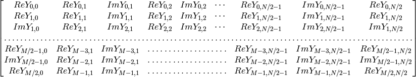
in the case of 1D transform of real vector, the output will look as the first row of the above matrix.
So, the function chooses the operation mode depending on the flags and size of the input array:
- if DFT_ROWS is set or the input array has single row or single column then the function performs 1D forward or inverse transform (of each row of a matrix when DFT_ROWS is set, otherwise it will be 2D transform.
- if input array is real and
DFT_INVERSE
is not set, the function does forward 1D or 2D transform:
- when DFT_COMPLEX_OUTPUT is set then the output will be complex matrix of the same size as input.
- otherwise the output will be a real matrix of the same size as input. in the case of 2D transform it will use the packed format as shown above; in the case of single 1D transform it will look as the first row of the above matrix; in the case of multiple 1D transforms (when using DCT_ROWS flag) each row of the output matrix will look like the first row of the above matrix.
- otherwise, if the input array is complex and either DFT_INVERSE or DFT_REAL_OUTPUT are not set then the output will be a complex array of the same size as input and the function will perform the forward or inverse 1D or 2D transform of the whole input array or each row of the input array independently, depending on the flags DFT_INVERSE and DFT_ROWS .
- otherwise, i.e. when DFT_INVERSE is set, the input array is real, or it is complex but DFT_REAL_OUTPUT is set, the output will be a real array of the same size as input, and the function will perform 1D or 2D inverse transformation of the whole input array or each individual row, depending on the flags DFT_INVERSE and DFT_ROWS .
The scaling is done after the transformation if DFT_SCALE is set.
Unlike dct() , the function supports arrays of arbitrary size, but only those arrays are processed efficiently, which sizes can be factorized in a product of small prime numbers (2, 3 and 5 in the current implementation). Such an efficient DFT size can be computed using getOptimalDFTSize() method.
Here is the sample on how to compute DFT-based convolution of two 2D real arrays:
void convolveDFT(const Mat& A, const Mat& B, Mat& C)
{
    // reallocate the output array if needed
    C.create(abs(A.rows - B.rows)+1, abs(A.cols - B.cols)+1, A.type());
    Size dftSize;
    // compute the size of DFT transform
    dftSize.width = getOptimalDFTSize(A.cols + B.cols - 1);
    dftSize.height = getOptimalDFTSize(A.rows + B.rows - 1);

    // allocate temporary buffers and initialize them with 0's
    Mat tempA(dftSize, A.type(), Scalar::all(0));
    Mat tempB(dftSize, B.type(), Scalar::all(0));

    // copy A and B to the top-left corners of tempA and tempB, respectively
    Mat roiA(tempA, Rect(0,0,A.cols,A.rows));
    A.copyTo(roiA);
    Mat roiB(tempB, Rect(0,0,B.cols,B.rows));
    B.copyTo(roiB);

    // now transform the padded A & B in-place;
    // use "nonzeroRows" hint for faster processing
    dft(tempA, tempA, 0, A.rows);
    dft(tempB, tempB, 0, B.rows);

    // multiply the spectrums;
    // the function handles packed spectrum representations well
    mulSpectrums(tempA, tempB, tempA);

    // transform the product back from the frequency domain.
    // Even though all the result rows will be non-zero,
    // we need only the first C.rows of them, and thus we
    // pass nonzeroRows == C.rows
    dft(tempA, tempA, DFT_INVERSE + DFT_SCALE, C.rows);

    // now copy the result back to C.
    tempA(Rect(0, 0, C.cols, C.rows)).copyTo(C);

    // all the temporary buffers will be deallocated automatically
}
What can be optimized in the above sample?
since we passed
 to the forward transform calls and
since we copied
A / B to the top-left corners of tempA / tempB , respectively,
it’s not necessary to clear the whole
tempA and tempB ;
it is only necessary to clear the
tempA.cols - A.cols ( tempB.cols - B.cols )
rightmost columns of the matrices.
- this DFT-based convolution does not have to be applied to the whole big arrays,
especially if
B is significantly smaller than A or vice versa.
Instead, we can compute convolution by parts. For that we need to split the destination array
C into multiple tiles and for each tile estimate, which parts of A and B are required to compute convolution in this tile. If the tiles in C are too small,
the speed will decrease a lot, because of repeated work - in the ultimate case, when each tile in
C is a single pixel,
the algorithm becomes equivalent to the naive convolution algorithm. If the tiles are too big, the temporary arrays
tempA and tempB become too big
and there is also slowdown because of bad cache locality. So there is optimal tile size somewhere in the middle.
if the convolution is done by parts, since different tiles in C can be computed in parallel, the loop can be threaded.
All of the above improvements have been implemented in matchTemplate() and filter2D() , therefore, by using them, you can get even better performance than with the above theoretically optimal implementation (though, those two functions actually compute cross-correlation, not convolution, so you will need to “flip” the kernel or the image around the center using flip() ).
See also: dct() , getOptimalDFTSize() , mulSpectrums() , filter2D() , matchTemplate() , flip() , cartToPolar() , magnitude() , phase()
cv::divide
- void divide(const MatND& src1, const MatND& src2, MatND& dst, double scale=1)
- void divide(double scale, const MatND& src2, MatND& dst)
Performs per-element division of two arrays or a scalar by an array.
Parameters: - src1 – The first source array
- src2 – The second source array; should have the same size and same type as src1
- scale – Scale factor
- dst – The destination array; will have the same size and same type as src2
The functions divide divide one array by another:

or a scalar by array, when there is no src1 :

The result will have the same type as src1 . When src2(I)=0 , dst(I)=0 too.
See also: multiply() , add() , subtract() , Matrix Expressions
cv::determinant
- double determinant(const Mat& mtx)
Returns determinant of a square floating-point matrix.
Parameters: - mtx – The input matrix; must have CV_32FC1 or CV_64FC1 type and square size
The function determinant computes and returns determinant of the specified matrix. For small matrices ( mtx.cols=mtx.rows<=3 ) the direct method is used; for larger matrices the function uses LU factorization.
For symmetric positive-determined matrices, it is also possible to compute
SVD()
:
 and then calculate the determinant as a product of the diagonal elements of
 .
.
See also: SVD() , trace() , invert() , solve() , Matrix Expressions
cv::eigen
- bool eigen(const Mat& src, Mat& eigenvalues, Mat& eigenvectors, int lowindex=-1, int highindex=-1)
Computes eigenvalues and eigenvectors of a symmetric matrix.
Parameters: - src – The input matrix; must have CV_32FC1 or CV_64FC1 type, square size and be symmetric:

- eigenvalues – The output vector of eigenvalues of the same type as src ; The eigenvalues are stored in the descending order.
- eigenvectors – The output matrix of eigenvectors; It will have the same size and the same type as src ; The eigenvectors are stored as subsequent matrix rows, in the same order as the corresponding eigenvalues
- lowindex – Optional index of largest eigenvalue/-vector to calculate. (See below.)
- highindex – Optional index of smallest eigenvalue/-vector to calculate. (See below.)
- src – The input matrix; must have CV_32FC1 or CV_64FC1 type, square size and be symmetric:
The functions eigen compute just eigenvalues, or eigenvalues and eigenvectors of symmetric matrix src :
src*eigenvectors(i,:)' = eigenvalues(i)*eigenvectors(i,:)' (in MATLAB notation)
If either low- or highindex is supplied the other is required, too. Indexing is 0-based. Example: To calculate the largest eigenvector/-value set lowindex = highindex = 0. For legacy reasons this function always returns a square matrix the same size as the source matrix with eigenvectors and a vector the length of the source matrix with eigenvalues. The selected eigenvectors/-values are always in the first highindex - lowindex + 1 rows.
See also: SVD() , completeSymm() , PCA()
cv::exp
- void exp(const MatND& src, MatND& dst)
Calculates the exponent of every array element.
Parameters: - src – The source array
- dst – The destination array; will have the same size and same type as src
The function exp calculates the exponent of every element of the input array:
![\texttt{dst} [I] = e^{ \texttt{src} }(I)](_images/math/13e517b3da9ab628878368589320811cfd644cd0.png)
The maximum relative error is about
 for single-precision and less than
 for double-precision. Currently, the function converts denormalized values to zeros on output. Special values (NaN,
) are not handled.
for double-precision. Currently, the function converts denormalized values to zeros on output. Special values (NaN,
) are not handled.
See also: log() , cartToPolar() , polarToCart() , phase() , pow() , sqrt() , magnitude()
cv::extractImageCOI
- void extractImageCOI(const CvArr* src, Mat& dst, int coi=-1)
Extract the selected image channel
Parameters: - src – The source array. It should be a pointer to CvMat or IplImage
- dst – The destination array; will have single-channel, and the same size and the same depth as src
- coi – If the parameter is >=0 , it specifies the channel to extract; If it is <0 , src must be a pointer to IplImage with valid COI set - then the selected COI is extracted.
The function extractImageCOI is used to extract image COI from an old-style array and put the result to the new-style C++ matrix. As usual, the destination matrix is reallocated using Mat::create if needed.
To extract a channel from a new-style matrix, use mixChannels() or split() See also: mixChannels() , split() , merge() , cvarrToMat() , cvSetImageCOI() , cvGetImageCOI()
cv::fastAtan2
- float fastAtan2(float y, float x)
Calculates the angle of a 2D vector in degrees
Parameters: - x – x-coordinate of the vector
- y – y-coordinate of the vector
The function
fastAtan2
calculates the full-range angle of an input 2D vector. The angle is
measured in degrees and varies from
 to
to
 . The accuracy is about
 .
.
cv::flip
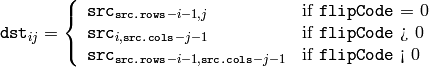
- void flip(const Mat& src, Mat& dst, int flipCode)
Flips a 2D array around vertical, horizontal or both axes.
Parameters: - src – The source array
- dst – The destination array; will have the same size and same type as src
- flipCode – Specifies how to flip the array: 0 means flipping around the x-axis, positive (e.g., 1) means flipping around y-axis, and negative (e.g., -1) means flipping around both axes. See also the discussion below for the formulas.
The function flip flips the array in one of three different ways (row and column indices are 0-based):
The example scenarios of function use are:
- vertical flipping of the image (
 ) to switch between top-left and bottom-left image origin, which is a typical operation in video processing in Windows.
 - horizontal flipping of the image with subsequent horizontal shift and absolute difference calculation to check for a vertical-axis symmetry (
 )
) - simultaneous horizontal and vertical flipping of the image with subsequent shift and absolute difference calculation to check for a central symmetry (
 )
) - reversing the order of 1d point arrays (
or
)
See also: transpose() , repeat() , completeSymm()
cv::gemm
- void gemm(const Mat& src1, const Mat& src2, double alpha, const Mat& src3, double beta, Mat& dst, int flags=0)
Performs generalized matrix multiplication.
Parameters: - src1 – The first multiplied input matrix; should have CV_32FC1 , CV_64FC1 , CV_32FC2 or CV_64FC2 type
- src2 – The second multiplied input matrix; should have the same type as src1
- alpha – The weight of the matrix product
- src3 – The third optional delta matrix added to the matrix product; should have the same type as src1 and src2
- beta – The weight of src3
- dst – The destination matrix; It will have the proper size and the same type as input matrices
- flags –
Operation flags:
- GEMM_1_T transpose src1
- GEMM_2_T transpose src2
- GEMM_3_T transpose src3
The function performs generalized matrix multiplication and similar to the corresponding functions *gemm in BLAS level 3. For example, gemm(src1, src2, alpha, src3, beta, dst, GEMM_1_T + GEMM_3_T) corresponds to

The function can be replaced with a matrix expression, e.g. the above call can be replaced with:
dst = alpha*src1.t()*src2 + beta*src3.t();
See also: mulTransposed() , transform() , Matrix Expressions
cv::getConvertElem
- ConvertData getConvertElem(int fromType, int toType)
- ConvertScaleData getConvertScaleElem(int fromType, int toType)
- typedef void (*ConvertData)(const void* from, void* to, int cn)
- typedef void (*ConvertScaleData)(const void* from, void* to, int cn, double alpha, double beta)
Returns conversion function for a single pixel
Parameters: - fromType – The source pixel type
- toType – The destination pixel type
- from – Callback parameter: pointer to the input pixel
- to – Callback parameter: pointer to the output pixel
- cn – Callback parameter: the number of channels; can be arbitrary, 1, 100, 100000, ...
- alpha – ConvertScaleData callback optional parameter: the scale factor
- beta – ConvertScaleData callback optional parameter: the delta or offset
The functions getConvertElem and getConvertScaleElem return pointers to the functions for converting individual pixels from one type to another. While the main function purpose is to convert single pixels (actually, for converting sparse matrices from one type to another), you can use them to convert the whole row of a dense matrix or the whole matrix at once, by setting cn = matrix.cols*matrix.rows*matrix.channels() if the matrix data is continuous.
See also: Mat::convertTo() , MatND::convertTo() , SparseMat::convertTo()
cv::getOptimalDFTSize
- int getOptimalDFTSize(int vecsize)
Returns optimal DFT size for a given vector size.
Parameters: - vecsize – Vector size
DFT performance is not a monotonic function of a vector size, therefore, when you compute convolution of two arrays or do a spectral analysis of array, it usually makes sense to pad the input data with zeros to get a bit larger array that can be transformed much faster than the original one. Arrays, which size is a power-of-two (2, 4, 8, 16, 32, ...) are the fastest to process, though, the arrays, which size is a product of 2’s, 3’s and 5’s (e.g. 300 = 5*5*3*2*2), are also processed quite efficiently.
The function
getOptimalDFTSize
returns the minimum number
N
that is greater than or equal to
vecsize
, such that the DFT
of a vector of size
N
can be computed efficiently. In the current implementation
 , for some
 ,
,
 ,
,
 .
.
The function returns a negative number if vecsize is too large (very close to INT_MAX ).
While the function cannot be used directly to estimate the optimal vector size for DCT transform (since the current DCT implementation supports only even-size vectors), it can be easily computed as getOptimalDFTSize((vecsize+1)/2)*2 .
See also: dft() , dct() , idft() , idct() , mulSpectrums()
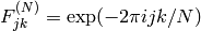
cv::idct
- void idct(const Mat& src, Mat& dst, int flags=0)
Computes inverse Discrete Cosine Transform of a 1D or 2D array
Parameters: - src – The source floating-point single-channel array
- dst – The destination array. Will have the same size and same type as src
- flags – The operation flags.
idct(src, dst, flags) is equivalent to dct(src, dst, flags | DCT_INVERSE) . See dct() for details.
See also: dct() , dft() , idft() , getOptimalDFTSize()
cv::idft
- void idft(const Mat& src, Mat& dst, int flags=0, int outputRows=0)
Computes inverse Discrete Fourier Transform of a 1D or 2D array
Parameters: - src – The source floating-point real or complex array
- dst – The destination array, which size and type depends on the flags
- flags – The operation flags. See dft()
- nonzeroRows – The number of dst rows to compute. The rest of the rows will have undefined content. See the convolution sample in dft() description
idft(src, dst, flags) is equivalent to dct(src, dst, flags | DFT_INVERSE) . See dft() for details. Note, that none of dft and idft scale the result by default. Thus, you should pass DFT_SCALE to one of dft or idft explicitly to make these transforms mutually inverse.
See also: dft() , dct() , idct() , mulSpectrums() , getOptimalDFTSize()
cv::inRange
- void inRange(const MatND& src, const MatND& lowerb, const MatND& upperb, MatND& dst)
- void inRange(const MatND& src, const Scalar& lowerb, const Scalar& upperb, MatND& dst)
Checks if array elements lie between the elements of two other arrays.
Parameters: - src – The first source array
- lowerb – The inclusive lower boundary array of the same size and type as src
- upperb – The exclusive upper boundary array of the same size and type as src
- dst – The destination array, will have the same size as src and CV_8U type
The functions inRange do the range check for every element of the input array:

for single-channel arrays,

for two-channel arrays and so forth. dst (I) is set to 255 (all 1 -bits) if src (I) is within the specified range and 0 otherwise.
cv::invert
- double invert(const Mat& src, Mat& dst, int method=DECOMP_LU)
Finds the inverse or pseudo-inverse of a matrix
Parameters: - src – The source floating-point matrix
- dst – The destination matrix; will have
 size and the same type as src
 - flags –
The inversion method :
- DECOMP_LU Gaussian elimination with optimal pivot element chosen
- DECOMP_SVD Singular value decomposition (SVD) method
- DECOMP_CHOLESKY Cholesky decomposion. The matrix must be symmetrical and positively defined
- src – The source floating-point
The function
invert
inverts matrix
src
and stores the result in
dst
.
When the matrix
src
is singular or non-square, the function computes the pseudo-inverse matrix, i.e. the matrix
dst
, such that
 is minimal.
In the case of DECOMP_LU method, the function returns the src determinant ( src must be square). If it is 0, the matrix is not inverted and dst is filled with zeros.
In the case of DECOMP_SVD method, the function returns the inversed condition number of src (the ratio of the smallest singular value to the largest singular value) and 0 if src is singular. The SVD method calculates a pseudo-inverse matrix if src is singular.
Similarly to DECOMP_LU , the method DECOMP_CHOLESKY works only with non-singular square matrices. In this case the function stores the inverted matrix in dst and returns non-zero, otherwise it returns 0.
See also: solve() , SVD()
cv::log
- void log(const MatND& src, MatND& dst)
Calculates the natural logarithm of every array element.
Parameters: - src – The source array
- dst – The destination array; will have the same size and same type as src
The function log calculates the natural logarithm of the absolute value of every element of the input array:
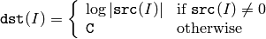
Where
C
is a large negative number (about -700 in the current implementation).
The maximum relative error is about
for single-precision input and less than
for double-precision input. Special values (NaN,
) are not handled.
See also: exp() , cartToPolar() , polarToCart() , phase() , pow() , sqrt() , magnitude()
cv::LUT
- void LUT(const Mat& src, const Mat& lut, Mat& dst)
Performs a look-up table transform of an array.
Parameters: - src – Source array of 8-bit elements
- lut – Look-up table of 256 elements. In the case of multi-channel source array, the table should either have a single channel (in this case the same table is used for all channels) or the same number of channels as in the source array
- dst – Destination array; will have the same size and the same number of channels as src , and the same depth as lut
The function LUT fills the destination array with values from the look-up table. Indices of the entries are taken from the source array. That is, the function processes each element of src as follows:

where
See also: convertScaleAbs() , Mat::convertTo
cv::magnitude
- void magnitude(const Mat& x, const Mat& y, Mat& magnitude)
Calculates magnitude of 2D vectors.
Parameters: - x – The floating-point array of x-coordinates of the vectors
- y – The floating-point array of y-coordinates of the vectors; must have the same size as x
- dst – The destination array; will have the same size and same type as x
The function magnitude calculates magnitude of 2D vectors formed from the corresponding elements of x and y arrays:
See also: cartToPolar() , polarToCart() , phase() , sqrt()
cv::Mahalanobis
- double Mahalanobis(const Mat& vec1, const Mat& vec2, const Mat& icovar)
Calculates the Mahalanobis distance between two vectors.
Parameters: - vec1 – The first 1D source vector
- vec2 – The second 1D source vector
- icovar – The inverse covariance matrix
The function cvMahalonobis calculates and returns the weighted distance between two vectors:

The covariance matrix may be calculated using the calcCovarMatrix() function and then inverted using the invert() function (preferably using DECOMP _ SVD method, as the most accurate).
cv::max
- Mat_Expr<...> max(const Mat& src1, double value)
- Mat_Expr<...> max(double value, const Mat& src1)
- void max(const MatND& src1, const MatND& src2, MatND& dst)
- void max(const MatND& src1, double value, MatND& dst)
Calculates per-element maximum of two arrays or array and a scalar
Parameters: - src1 – The first source array
- src2 – The second source array of the same size and type as src1
- value – The real scalar value
- dst – The destination array; will have the same size and type as src1
The functions max compute per-element maximum of two arrays:

or array and a scalar:

In the second variant, when the source array is multi-channel, each channel is compared with value independently.
The first 3 variants of the function listed above are actually a part of Matrix Expressions , they return the expression object that can be further transformed, or assigned to a matrix, or passed to a function etc.
See also: min() , compare() , inRange() , minMaxLoc() , Matrix Expressions
cv::mean
- Scalar mean(const MatND& mtx)
- Scalar mean(const MatND& mtx, const MatND& mask)
Calculates average (mean) of array elements
Parameters: - mtx – The source array; it should have 1 to 4 channels (so that the result can be stored in Scalar() )
- mask – The optional operation mask
The functions mean compute mean value M of array elements, independently for each channel, and return it:
When all the mask elements are 0’s, the functions return Scalar::all(0) .
See also: countNonZero() , meanStdDev() , norm() , minMaxLoc()
cv::meanStdDev
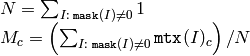
- void meanStdDev(const MatND& mtx, Scalar& mean, Scalar& stddev, const MatND& mask=MatND())
Calculates mean and standard deviation of array elements
Parameters: - mtx – The source array; it should have 1 to 4 channels (so that the results can be stored in Scalar() ‘s)
- mean – The output parameter: computed mean value
- stddev – The output parameter: computed standard deviation
- mask – The optional operation mask
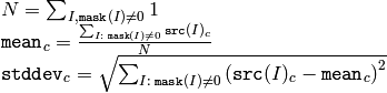
The functions meanStdDev compute the mean and the standard deviation M of array elements, independently for each channel, and return it via the output parameters:
When all the mask elements are 0’s, the functions return
mean=stddev=Scalar::all(0)
.
Note that the computed standard deviation is only the diagonal of the complete normalized covariance matrix. If the full matrix is needed, you can reshape the multi-channel array
to the single-channel array
 (only possible when the matrix is continuous) and then pass the matrix to
calcCovarMatrix()
.
(only possible when the matrix is continuous) and then pass the matrix to
calcCovarMatrix()
.
See also: countNonZero() , mean() , norm() , minMaxLoc() , calcCovarMatrix()
cv::merge
- void merge(const MatND* mv, size_t count, MatND& dst)
- void merge(const vector<MatND>& mv, MatND& dst)
Composes a multi-channel array from several single-channel arrays.
Parameters: - mv – The source array or vector of the single-channel matrices to be merged. All the matrices in mv must have the same size and the same type
- count – The number of source matrices when mv is a plain C array; must be greater than zero
- dst – The destination array; will have the same size and the same depth as mv[0] , the number of channels will match the number of source matrices
The functions merge merge several single-channel arrays (or rather interleave their elements) to make a single multi-channel array.
](_images/math/575eaf395d1f4af9ca3225e4b730c005049fb6fd.png)
The function split() does the reverse operation and if you need to merge several multi-channel images or shuffle channels in some other advanced way, use mixChannels() See also: mixChannels() , split() , reshape()
cv::min
- Mat_Expr<...> min(const Mat& src1, double value)
- Mat_Expr<...> min(double value, const Mat& src1)
- void min(const MatND& src1, const MatND& src2, MatND& dst)
- void min(const MatND& src1, double value, MatND& dst)
Calculates per-element minimum of two arrays or array and a scalar
Parameters: - src1 – The first source array
- src2 – The second source array of the same size and type as src1
- value – The real scalar value
- dst – The destination array; will have the same size and type as src1
The functions min compute per-element minimum of two arrays:

or array and a scalar:

In the second variant, when the source array is multi-channel, each channel is compared with value independently.
The first 3 variants of the function listed above are actually a part of Matrix Expressions , they return the expression object that can be further transformed, or assigned to a matrix, or passed to a function etc.
See also: max() , compare() , inRange() , minMaxLoc() , Matrix Expressions
cv::minMaxLoc
- void minMaxLoc(const Mat& src, double* minVal, double* maxVal=0, Point* minLoc=0, Point* maxLoc=0, const Mat& mask=Mat())
- void minMaxLoc(const MatND& src, double* minVal, double* maxVal, int* minIdx=0, int* maxIdx=0, const MatND& mask=MatND())
- void minMaxLoc(const SparseMat& src, double* minVal, double* maxVal, int* minIdx=0, int* maxIdx=0)
Finds global minimum and maximum in a whole array or sub-array
Parameters: - src – The source single-channel array
- minVal – Pointer to returned minimum value; NULL if not required
- maxVal – Pointer to returned maximum value; NULL if not required
- minLoc – Pointer to returned minimum location (in 2D case); NULL if not required
- maxLoc – Pointer to returned maximum location (in 2D case); NULL if not required
- minIdx – Pointer to returned minimum location (in nD case); NULL if not required, otherwise must point to an array of src.dims elements and the coordinates of minimum element in each dimensions will be stored sequentially there.
- maxIdx – Pointer to returned maximum location (in nD case); NULL if not required
- mask – The optional mask used to select a sub-array
The functions ninMaxLoc find minimum and maximum element values and their positions. The extremums are searched across the whole array, or, if mask is not an empty array, in the specified array region.
The functions do not work with multi-channel arrays. If you need to find minimum or maximum elements across all the channels, use reshape() first to reinterpret the array as single-channel. Or you may extract the particular channel using extractImageCOI() or mixChannels() or split() .
in the case of a sparse matrix the minimum is found among non-zero elements only.
See also: max() , min() , compare() , inRange() , extractImageCOI() , mixChannels() , split() , reshape() .
cv::mixChannels
- void mixChannels(const MatND* srcv, int nsrc, MatND* dstv, int ndst, const int* fromTo, size_t npairs)
- void mixChannels(const vector<MatND>& srcv, vector<MatND>& dstv, const int* fromTo, int npairs)
Copies specified channels from input arrays to the specified channels of output arrays
Parameters: - srcv – The input array or vector of matrices. All the matrices must have the same size and the same depth
- nsrc – The number of elements in srcv
- dstv – The output array or vector of matrices. All the matrices must be allocated , their size and depth must be the same as in srcv[0]
- ndst – The number of elements in dstv
- fromTo – The array of index pairs, specifying which channels are copied and where. fromTo[k*2] is the 0-based index of the input channel in srcv and fromTo[k*2+1] is the index of the output channel in dstv . Here the continuous channel numbering is used, that is, the first input image channels are indexed from 0 to srcv[0].channels()-1 , the second input image channels are indexed from srcv[0].channels() to srcv[0].channels() + srcv[1].channels()-1 etc., and the same scheme is used for the output image channels. As a special case, when fromTo[k*2] is negative, the corresponding output channel is filled with zero.
npairs
The functions mixChannels provide an advanced mechanism for shuffling image channels. split() and merge() and some forms of cvtColor() are partial cases of mixChannels .
As an example, this code splits a 4-channel RGBA image into a 3-channel BGR (i.e. with R and B channels swapped) and separate alpha channel image:
Mat rgba( 100, 100, CV_8UC4, Scalar(1,2,3,4) );
Mat bgr( rgba.rows, rgba.cols, CV_8UC3 );
Mat alpha( rgba.rows, rgba.cols, CV_8UC1 );

// forming array of matrices is quite efficient operations,
// because the matrix data is not copied, only the headers
Mat out[] = { bgr, alpha };
// rgba[0] -> bgr[2], rgba[1] -> bgr[1],
// rgba[2] -> bgr[0], rgba[3] -> alpha[0]
int from_to[] = { 0,2,  1,1,  2,0,  3,3 };
mixChannels( &rgba, 1, out, 2, from_to, 4 );
Note that, unlike many other new-style C++ functions in OpenCV (see the introduction section and Mat::create() ), mixChannels requires the destination arrays be pre-allocated before calling the function.
See also: split() , merge() , cvtColor()
cv::mulSpectrums
- void mulSpectrums(const Mat& src1, const Mat& src2, Mat& dst, int flags, bool conj=false)
Performs per-element multiplication of two Fourier spectrums.
Parameters: - src1 – The first source array
- src2 – The second source array; must have the same size and the same type as src1
- dst – The destination array; will have the same size and the same type as src1
- flags – The same flags as passed to dft() ; only the flag DFT_ROWS is checked for
- conj – The optional flag that conjugate the second source array before the multiplication (true) or not (false)
The function mulSpectrums performs per-element multiplication of the two CCS-packed or complex matrices that are results of a real or complex Fourier transform.
The function, together with dft() and idft() , may be used to calculate convolution (pass conj=false ) or correlation (pass conj=false ) of two arrays rapidly. When the arrays are complex, they are simply multiplied (per-element) with optional conjugation of the second array elements. When the arrays are real, they assumed to be CCS-packed (see dft() for details).
cv::multiply
- void multiply(const MatND& src1, const MatND& src2, MatND& dst, double scale=1)
Calculates the per-element scaled product of two arrays
Parameters: - src1 – The first source array
- src2 – The second source array of the same size and the same type as src1
- dst – The destination array; will have the same size and the same type as src1
- scale – The optional scale factor
The function multiply calculates the per-element product of two arrays:

There is also Matrix Expressions -friendly variant of the first function, see Mat::mul() .
If you are looking for a matrix product, not per-element product, see gemm() .
See also: add() , substract() , divide() , Matrix Expressions , scaleAdd() , addWeighted() , accumulate() , accumulateProduct() , accumulateSquare() , Mat::convertTo()
cv::mulTransposed
- void mulTransposed(const Mat& src, Mat& dst, bool aTa, const Mat& delta=Mat(), double scale=1, int rtype=-1)
Calculates the product of a matrix and its transposition.
Parameters: - src – The source matrix
- dst – The destination square matrix
- aTa – Specifies the multiplication ordering; see the description below
- delta – The optional delta matrix, subtracted from src before the multiplication. When the matrix is empty ( delta=Mat() ), it’s assumed to be zero, i.e. nothing is subtracted, otherwise if it has the same size as src , then it’s simply subtracted, otherwise it is “repeated” (see repeat() ) to cover the full src and then subtracted. Type of the delta matrix, when it’s not empty, must be the same as the type of created destination matrix, see the rtype description
- scale – The optional scale factor for the matrix product
- rtype – When it’s negative, the destination matrix will have the same type as src . Otherwise, it will have type=CV_MAT_DEPTH(rtype) , which should be either CV_32F or CV_64F
The function mulTransposed calculates the product of src and its transposition:

if aTa=true , and

otherwise. The function is used to compute covariance matrix and with zero delta can be used as a faster substitute for general matrix product
 when
when
 .
.
See also: calcCovarMatrix() , gemm() , repeat() , reduce()
cv::norm
- double norm(const MatND& src1, int normType=NORM_L2, const MatND& mask=MatND())
- double norm(const MatND& src1, const MatND& src2, int normType=NORM_L2, const MatND& mask=MatND())
- double norm(const SparseMat& src, int normType)
Calculates absolute array norm, absolute difference norm, or relative difference norm.
Parameters: - src1 – The first source array
- src2 – The second source array of the same size and the same type as src1
- normType – Type of the norm; see the discussion below
- mask – The optional operation mask
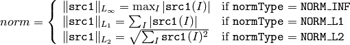
The functions norm calculate the absolute norm of src1 (when there is no src2 ):
or an absolute or relative difference norm if src2 is there:
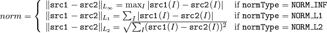
or
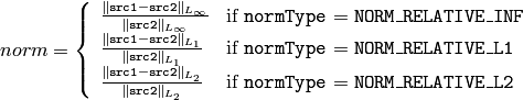
The functions norm return the calculated norm.
When there is mask parameter, and it is not empty (then it should have type CV_8U and the same size as src1 ), the norm is computed only over the specified by the mask region.
A multiple-channel source arrays are treated as a single-channel, that is, the results for all channels are combined.
cv::normalize
- void normalize(const Mat& src, Mat& dst, double alpha=1, double beta=0, int normType=NORM_L2, int rtype=-1, const Mat& mask=Mat())
- void normalize(const MatND& src, MatND& dst, double alpha=1, double beta=0, int normType=NORM_L2, int rtype=-1, const MatND& mask=MatND())
- void normalize(const SparseMat& src, SparseMat& dst, double alpha, int normType)
Normalizes array’s norm or the range
Parameters: - src – The source array
- dst – The destination array; will have the same size as src
- alpha – The norm value to normalize to or the lower range boundary in the case of range normalization
- beta – The upper range boundary in the case of range normalization; not used for norm normalization
- normType – The normalization type, see the discussion
- rtype – When the parameter is negative, the destination array will have the same type as src , otherwise it will have the same number of channels as src and the depth =CV_MAT_DEPTH(rtype)
- mask – The optional operation mask
The functions normalize scale and shift the source array elements, so that

(where
 , 1 or 2) when
normType=NORM_INF
,
NORM_L1
or
NORM_L2
,
or so that
, 1 or 2) when
normType=NORM_INF
,
NORM_L1
or
NORM_L2
,
or so that

when normType=NORM_MINMAX (for dense arrays only).
The optional mask specifies the sub-array to be normalize, that is, the norm or min-n-max are computed over the sub-array and then this sub-array is modified to be normalized. If you want to only use the mask to compute the norm or min-max, but modify the whole array, you can use norm() and Mat::convertScale() / MatND::convertScale() /cross{SparseMat::convertScale} separately.
in the case of sparse matrices, only the non-zero values are analyzed and transformed. Because of this, the range transformation for sparse matrices is not allowed, since it can shift the zero level.
See also: norm() , Mat::convertScale() , MatND::convertScale() , SparseMat::convertScale()
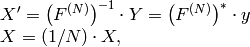
PCA
- PCA
Class for Principal Component Analysis
class PCA
{
public:
    // default constructor
    PCA();
    // computes PCA for a set of vectors stored as data rows or columns.
    PCA(const Mat& data, const Mat& mean, int flags, int maxComponents=0);
    // computes PCA for a set of vectors stored as data rows or columns
    PCA& operator()(const Mat& data, const Mat& mean, int flags, int maxComponents=0);
    // projects vector into the principal components space
    Mat project(const Mat& vec) const;
    void project(const Mat& vec, Mat& result) const;
    // reconstructs the vector from its PC projection
    Mat backProject(const Mat& vec) const;
    void backProject(const Mat& vec, Mat& result) const;

    // eigenvectors of the PC space, stored as the matrix rows
    Mat eigenvectors;
    // the corresponding eigenvalues; not used for PCA compression/decompression
    Mat eigenvalues;
    // mean vector, subtracted from the projected vector
    // or added to the reconstructed vector
    Mat mean;
};
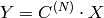
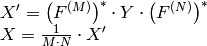
The class PCA is used to compute the special basis for a set of vectors. The basis will consist of eigenvectors of the covariance matrix computed from the input set of vectors. And also the class PCA can transform vectors to/from the new coordinate space, defined by the basis. Usually, in this new coordinate system each vector from the original set (and any linear combination of such vectors) can be quite accurately approximated by taking just the first few its components, corresponding to the eigenvectors of the largest eigenvalues of the covariance matrix. Geometrically it means that we compute projection of the vector to a subspace formed by a few eigenvectors corresponding to the dominant eigenvalues of the covariation matrix. And usually such a projection is very close to the original vector. That is, we can represent the original vector from a high-dimensional space with a much shorter vector consisting of the projected vector’s coordinates in the subspace. Such a transformation is also known as Karhunen-Loeve Transform, or KLT. See http://en.wikipedia.org/wiki/Principal_component_analysis The following sample is the function that takes two matrices. The first one stores the set of vectors (a row per vector) that is used to compute PCA, the second one stores another “test” set of vectors (a row per vector) that are first compressed with PCA, then reconstructed back and then the reconstruction error norm is computed and printed for each vector.
PCA compressPCA(const Mat& pcaset, int maxComponents,
                const Mat& testset, Mat& compressed)
{
    PCA pca(pcaset, // pass the data
            Mat(), // we do not have a pre-computed mean vector,
                   // so let the PCA engine to compute it
            CV_PCA_DATA_AS_ROW, // indicate that the vectors
                                // are stored as matrix rows
                                // (use CV_PCA_DATA_AS_COL if the vectors are
                                // the matrix columns)
            maxComponents // specify, how many principal components to retain
            );
    // if there is no test data, just return the computed basis, ready-to-use
    if( !testset.data )
        return pca;
    CV_Assert( testset.cols == pcaset.cols );

    compressed.create(testset.rows, maxComponents, testset.type());

    Mat reconstructed;
    for( int i = 0; i < testset.rows; i++ )
    {
        Mat vec = testset.row(i), coeffs = compressed.row(i);
        // compress the vector, the result will be stored
        // in the i-th row of the output matrix
        pca.project(vec, coeffs);
        // and then reconstruct it
        pca.backProject(coeffs, reconstructed);
        // and measure the error
        printf("
    }
    return pca;
}
See also: calcCovarMatrix() , mulTransposed() , SVD() , dft() , dct()
cv::PCA::PCA
- PCA::PCA()
- PCA::PCA(const Mat& data, const Mat& mean, int flags, int maxComponents=0)
PCA constructors
Parameters: - data – the input samples, stored as the matrix rows or as the matrix columns
- mean – the optional mean value. If the matrix is empty ( Mat() ), the mean is computed from the data.
- flags –
operation flags. Currently the parameter is only used to specify the data layout.
- CV_PCA_DATA_AS_ROWS Indicates that the input samples are stored as matrix rows.
- CV_PCA_DATA_AS_COLS Indicates that the input samples are stored as matrix columns.
- maxComponents – The maximum number of components that PCA should retain. By default, all the components are retained.
The default constructor initializes empty PCA structure. The second constructor initializes the structure and calls PCA::operator () .
cv::PCA::operator ()
- PCA& PCA::operator()(const Mat& data, const Mat& mean, int flags, int maxComponents=0)
Performs Principal Component Analysis of the supplied dataset.
Parameters: - data – the input samples, stored as the matrix rows or as the matrix columns
- mean – the optional mean value. If the matrix is empty ( Mat() ), the mean is computed from the data.
- flags –
operation flags. Currently the parameter is only used to specify the data layout.
- CV_PCA_DATA_AS_ROWS Indicates that the input samples are stored as matrix rows.
- CV_PCA_DATA_AS_COLS Indicates that the input samples are stored as matrix columns.
- maxComponents – The maximum number of components that PCA should retain. By default, all the components are retained.
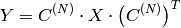
The operator performs PCA of the supplied dataset. It is safe to reuse the same PCA structure for multiple dataset. That is, if the structure has been previously used with another dataset, the existing internal data is reclaimed and the new eigenvalues , eigenvectors and mean are allocated and computed.
The computed eigenvalues are sorted from the largest to the smallest and the corresponding eigenvectors are stored as PCA::eigenvectors rows.
cv::PCA::project
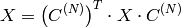
- void PCA::project(const Mat& vec, Mat& result) const
Project vector(s) to the principal component subspace
Parameters: - vec – the input vector(s). They have to have the same dimensionality and the same layout as the input data used at PCA phase. That is, if CV_PCA_DATA_AS_ROWS had been specified, then vec.cols==data.cols (that’s vectors’ dimensionality) and vec.rows is the number of vectors to project; and similarly for the CV_PCA_DATA_AS_COLS case.
- result – the output vectors. Let’s now consider CV_PCA_DATA_AS_COLS case. In this case the output matrix will have as many columns as the number of input vectors, i.e. result.cols==vec.cols and the number of rows will match the number of principal components (e.g. maxComponents parameter passed to the constructor).
The methods project one or more vectors to the principal component subspace, where each vector projection is represented by coefficients in the principal component basis. The first form of the method returns the matrix that the second form writes to the result. So the first form can be used as a part of expression, while the second form can be more efficient in a processing loop.
cv::PCA::backProject
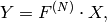
- void PCA::backProject(const Mat& vec, Mat& result) const
Reconstruct vectors from their PC projections.
Parameters: - vec – Coordinates of the vectors in the principal component subspace. The layout and size are the same as of PCA::project output vectors.
- result – The reconstructed vectors. The layout and size are the same as of PCA::project input vectors.
The methods are inverse operations to PCA::project() . They take PC coordinates of projected vectors and reconstruct the original vectors. Of course, unless all the principal components have been retained, the reconstructed vectors will be different from the originals, but typically the difference will be small is if the number of components is large enough (but still much smaller than the original vector dimensionality) - that’s why PCA is used after all.
cv::perspectiveTransform
- void perspectiveTransform(const Mat& src, Mat& dst, const Mat& mtx)
Performs perspective matrix transformation of vectors.
Parameters: - src – The source two-channel or three-channel floating-point array; each element is 2D/3D vector to be transformed
- dst – The destination array; it will have the same size and same type as src
- mtx –
 or
or  transformation matrix
The function
perspectiveTransform
transforms every element of
src
,
by treating it as 2D or 3D vector, in the following way (here 3D vector transformation is shown; in the case of 2D vector transformation the
 component is omitted):

where

and
Note that the function transforms a sparse set of 2D or 3D vectors. If you want to transform an image using perspective transformation, use warpPerspective() . If you have an inverse task, i.e. want to compute the most probable perspective transformation out of several pairs of corresponding points, you can use getPerspectiveTransform() or findHomography() .
See also: transform() , warpPerspective() , getPerspectiveTransform() , findHomography()
cv::phase
- void phase(const Mat& x, const Mat& y, Mat& angle, bool angleInDegrees=false)
Calculates the rotation angle of 2d vectors
Parameters: - x – The source floating-point array of x-coordinates of 2D vectors
- y – The source array of y-coordinates of 2D vectors; must have the same size and the same type as x
- angle – The destination array of vector angles; it will have the same size and same type as x
- angleInDegrees – When it is true, the function will compute angle in degrees, otherwise they will be measured in radians
The function phase computes the rotation angle of each 2D vector that is formed from the corresponding elements of x and y :

The angle estimation accuracy is
, when
x(I)=y(I)=0
, the corresponding
angle
(I) is set to
 .
.
See also:
cv::polarToCart
- void polarToCart(const Mat& magnitude, const Mat& angle, Mat& x, Mat& y, bool angleInDegrees=false)
Computes x and y coordinates of 2D vectors from their magnitude and angle.
Parameters: - magnitude – The source floating-point array of magnitudes of 2D vectors. It can be an empty matrix ( =Mat() ) - in this case the function assumes that all the magnitudes are =1. If it’s not empty, it must have the same size and same type as angle
- angle – The source floating-point array of angles of the 2D vectors
- x – The destination array of x-coordinates of 2D vectors; will have the same size and the same type as angle
- y – The destination array of y-coordinates of 2D vectors; will have the same size and the same type as angle
- angleInDegrees – When it is true, the input angles are measured in degrees, otherwise they are measured in radians
The function polarToCart computes the cartesian coordinates of each 2D vector represented by the corresponding elements of magnitude and angle :
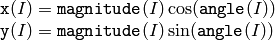
The relative accuracy of the estimated coordinates is
 .
.
See also: cartToPolar() , magnitude() , phase() , exp() , log() , pow() , sqrt()
cv::pow
- void pow(const MatND& src, double p, MatND& dst)
Raises every array element to a power.
Parameters: - src – The source array
- p – The exponent of power
- dst – The destination array; will have the same size and the same type as src
The function pow raises every element of the input array to p :
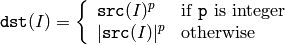
That is, for a non-integer power exponent the absolute values of input array elements are used. However, it is possible to get true values for negative values using some extra operations, as the following example, computing the 5th root of array src , shows:
Mat mask = src < 0;
pow(src, 1./5, dst);
subtract(Scalar::all(0), dst, dst, mask);
For some values of p , such as integer values, 0.5, and -0.5, specialized faster algorithms are used.
See also: sqrt() , exp() , log() , cartToPolar() , polarToCart()
RNG
Random number generator class.
class CV_EXPORTS RNG
{
public:
    enum { A=4164903690U, UNIFORM=0, NORMAL=1 };

    // constructors
    RNG();
    RNG(uint64 state);

    // returns 32-bit unsigned random number
    unsigned next();

    // return random numbers of the specified type
    operator uchar();
    operator schar();
    operator ushort();
    operator short();
    operator unsigned();
        // returns a random integer sampled uniformly from [0, N).
        unsigned operator()(unsigned N);
        unsigned operator()();
    operator int();
    operator float();
    operator double();
    // returns a random number sampled uniformly from [a, b) range
    int uniform(int a, int b);
    float uniform(float a, float b);
    double uniform(double a, double b);

    // returns Gaussian random number with zero mean.
        double gaussian(double sigma);

    // fills array with random numbers sampled from the specified distribution
    void fill( Mat& mat, int distType, const Scalar& a, const Scalar& b );
    void fill( MatND& mat, int distType, const Scalar& a, const Scalar& b );

    // internal state of the RNG (could change in the future)
    uint64 state;
};
The class RNG implements random number generator. It encapsulates the RNG state (currently, a 64-bit integer) and has methods to return scalar random values and to fill arrays with random values. Currently it supports uniform and Gaussian (normal) distributions. The generator uses Multiply-With-Carry algorithm, introduced by G. Marsaglia ( http://en.wikipedia.org/wiki/Multiply-with-carry ). Gaussian-distribution random numbers are generated using Ziggurat algorithm ( http://en.wikipedia.org/wiki/Ziggurat_algorithm ), introduced by G. Marsaglia and W. W. Tsang.
cv::RNG::RNG
- RNG::RNG()
- RNG::RNG(uint64 state)
RNG constructors
Parameters: - state – the 64-bit value used to initialize the RNG
These are the RNG constructors. The first form sets the state to some pre-defined value, equal to 2**32-1 in the current implementation. The second form sets the state to the specified value. If the user passed state=0 , the constructor uses the above default value instead, to avoid the singular random number sequence, consisting of all zeros.
cv::RNG::next
- unsigned RNG::next()
Returns the next random number
The method updates the state using MWC algorithm and returns the next 32-bit random number.
cv::RNG::operator T
- RNG::operator uchar() RNG::operator schar() RNG::operator ushort() RNG::operator short() RNG::operator unsigned() RNG::operator int() RNG::operator float() RNG::operator double()
Returns the next random number of the specified type
Each of the methods updates the state using MWC algorithm and returns the next random number of the specified type. In the case of integer types the returned number is from the whole available value range for the specified type. In the case of floating-point types the returned value is from [0,1) range.
cv::RNG::operator ()
- unsigned RNG::operator()()
- unsigned RNG::operator()(unsigned N)
Returns the next random number
Parameters: - N – The upper non-inclusive boundary of the returned random number
The methods transforms the state using MWC algorithm and returns the next random number. The first form is equivalent to RNG::next() , the second form returns the random number modulo N , i.e. the result will be in the range [0, N) .
cv::RNG::uniform
- int RNG::uniform(int a, int b)
- float RNG::uniform(float a, float b)
- double RNG::uniform(double a, double b)
Returns the next random number sampled from the uniform distribution
Parameters: - a – The lower inclusive boundary of the returned random numbers
- b – The upper non-inclusive boundary of the returned random numbers
The methods transforms the state using MWC algorithm and returns the next uniformly-distributed random number of the specified type, deduced from the input parameter type, from the range [a, b) . There is one nuance, illustrated by the following sample:
cv::RNG rng;

// will always produce 0
double a = rng.uniform(0, 1);

// will produce double from [0, 1)
double a1 = rng.uniform((double)0, (double)1);

// will produce float from [0, 1)
double b = rng.uniform(0.f, 1.f);

// will produce double from [0, 1)
double c = rng.uniform(0., 1.);

// will likely cause compiler error because of ambiguity:
//  RNG::uniform(0, (int)0.999999)? or RNG::uniform((double)0, 0.99999)?
double d = rng.uniform(0, 0.999999);
That is, the compiler does not take into account type of the variable that you assign the result of RNG::uniform to, the only thing that matters to it is the type of a and b parameters. So if you want a floating-point random number, but the range boundaries are integer numbers, either put dots in the end, if they are constants, or use explicit type cast operators, as in a1 initialization above.
cv::RNG::gaussian
- double RNG::gaussian(double sigma)
Returns the next random number sampled from the Gaussian distribution
Parameters: - sigma – The standard deviation of the distribution
The methods transforms the state using MWC algorithm and returns the next random number from the Gaussian distribution N(0,sigma) . That is, the mean value of the returned random numbers will be zero and the standard deviation will be the specified sigma .
cv::RNG::fill
- void RNG::fill(MatND& mat, int distType, const Scalar& a, const Scalar& b)
Fill arrays with random numbers
Parameters: - mat – 2D or N-dimensional matrix. Currently matrices with more than 4 channels are not supported by the methods. Use reshape() as a possible workaround.
- distType – The distribution type, RNG::UNIFORM or RNG::NORMAL
- a – The first distribution parameter. In the case of uniform distribution this is inclusive lower boundary. In the case of normal distribution this is mean value.
- b – The second distribution parameter. In the case of uniform distribution this is non-inclusive upper boundary. In the case of normal distribution this is standard deviation.
Each of the methods fills the matrix with the random values from the specified distribution. As the new numbers are generated, the RNG state is updated accordingly. In the case of multiple-channel images every channel is filled independently, i.e. RNG can not generate samples from multi-dimensional Gaussian distribution with non-diagonal covariation matrix directly. To do that, first, generate matrix from the distribution
 , i.e. Gaussian distribution with zero mean and identity covariation matrix, and then transform it using
transform()
and the specific covariation matrix.
, i.e. Gaussian distribution with zero mean and identity covariation matrix, and then transform it using
transform()
and the specific covariation matrix.
cv::randu
- template<typename _Tp> _Tp randu()
- void randu(Mat& mtx, const Scalar& low, const Scalar& high)
Generates a single uniformly-distributed random number or array of random numbers
Parameters: - mtx – The output array of random numbers. The array must be pre-allocated and have 1 to 4 channels
- low – The inclusive lower boundary of the generated random numbers
- high – The exclusive upper boundary of the generated random numbers
The template functions randu generate and return the next uniformly-distributed random value of the specified type. randu<int>() is equivalent to (int)theRNG(); etc. See RNG() description.
The second non-template variant of the function fills the matrix mtx with uniformly-distributed random numbers from the specified range:

See also: RNG() , randn() , theRNG() .
cv::randn
- void randn(Mat& mtx, const Scalar& mean, const Scalar& stddev)
Fills array with normally distributed random numbers
Parameters: - mtx – The output array of random numbers. The array must be pre-allocated and have 1 to 4 channels
- mean – The mean value (expectation) of the generated random numbers
- stddev – The standard deviation of the generated random numbers
The function randn fills the matrix mtx with normally distributed random numbers with the specified mean and standard deviation. is applied to the generated numbers (i.e. the values are clipped)
See also: RNG() , randu()
cv::randShuffle
- void randShuffle(Mat& mtx, double iterFactor=1., RNG* rng=0)
Shuffles the array elements randomly
Parameters: - mtx – The input/output numerical 1D array
- iterFactor – The scale factor that determines the number of random swap operations. See the discussion
- rng – The optional random number generator used for shuffling. If it is zero, theRNG() () is used instead
The function randShuffle shuffles the specified 1D array by randomly choosing pairs of elements and swapping them. The number of such swap operations will be mtx.rows*mtx.cols*iterFactor See also: RNG() , sort()
cv::reduce
- void reduce(const Mat& mtx, Mat& vec, int dim, int reduceOp, int dtype=-1)
Reduces a matrix to a vector
Parameters: - mtx – The source 2D matrix
- vec – The destination vector. Its size and type is defined by dim and dtype parameters
- dim – The dimension index along which the matrix is reduced. 0 means that the matrix is reduced to a single row and 1 means that the matrix is reduced to a single column
- reduceOp –
The reduction operation, one of:
- CV_REDUCE_SUM The output is the sum of all of the matrix’s rows/columns.
- CV_REDUCE_AVG The output is the mean vector of all of the matrix’s rows/columns.
- CV_REDUCE_MAX The output is the maximum (column/row-wise) of all of the matrix’s rows/columns.
- CV_REDUCE_MIN The output is the minimum (column/row-wise) of all of the matrix’s rows/columns.
- dtype – When it is negative, the destination vector will have the same type as the source matrix, otherwise, its type will be CV_MAKE_TYPE(CV_MAT_DEPTH(dtype), mtx.channels())
The function reduce reduces matrix to a vector by treating the matrix rows/columns as a set of 1D vectors and performing the specified operation on the vectors until a single row/column is obtained. For example, the function can be used to compute horizontal and vertical projections of an raster image. In the case of CV_REDUCE_SUM and CV_REDUCE_AVG the output may have a larger element bit-depth to preserve accuracy. And multi-channel arrays are also supported in these two reduction modes.
See also: repeat()
cv::repeat
- Mat repeat(const Mat& src, int ny, int nx)
Fill the destination array with repeated copies of the source array.
Parameters: - src – The source array to replicate
- dst – The destination array; will have the same type as src
- ny – How many times the src is repeated along the vertical axis
- nx – How many times the src is repeated along the horizontal axis
The functions repeat() duplicate the source array one or more times along each of the two axes:

The second variant of the function is more convenient to use with Matrix Expressions See also: reduce() , Matrix Expressions
saturate_cast
- template<typename _Tp> inline _Tp saturate_cast(unsigned char v)
- template<typename _Tp> inline _Tp saturate_cast(signed char v)
- template<typename _Tp> inline _Tp saturate_cast(unsigned short v)
- template<typename _Tp> inline _Tp saturate_cast(signed short v)
- template<typename _Tp> inline _Tp saturate_cast(int v)
- template<typename _Tp> inline _Tp saturate_cast(unsigned int v)
- template<typename _Tp> inline _Tp saturate_cast(float v)
- template<typename _Tp> inline _Tp saturate_cast(double v)
Template function for accurate conversion from one primitive type to another
Parameters: - v – The function parameter
The functions saturate_cast resembles the standard C++ cast operations, such as static_cast<T>() etc. They perform an efficient and accurate conversion from one primitive type to another, see the introduction. “saturate” in the name means that when the input value v is out of range of the target type, the result will not be formed just by taking low bits of the input, but instead the value will be clipped. For example:
uchar a = saturate_cast<uchar>(-100); // a = 0 (UCHAR_MIN)
short b = saturate_cast<short>(33333.33333); // b = 32767 (SHRT_MAX)
Such clipping is done when the target type is unsigned char, signed char, unsigned short or signed short - for 32-bit integers no clipping is done.
When the parameter is floating-point value and the target type is an integer (8-, 16- or 32-bit), the floating-point value is first rounded to the nearest integer and then clipped if needed (when the target type is 8- or 16-bit).
This operation is used in most simple or complex image processing functions in OpenCV.
See also: add() , subtract() , multiply() , divide() , Mat::convertTo()
cv::scaleAdd
- void scaleAdd(const MatND& src1, double scale, const MatND& src2, MatND& dst)
Calculates the sum of a scaled array and another array.
Parameters: - src1 – The first source array
- scale – Scale factor for the first array
- src2 – The second source array; must have the same size and the same type as src1
- dst – The destination array; will have the same size and the same type as src1
The function cvScaleAdd is one of the classical primitive linear algebra operations, known as DAXPY or SAXPY in BLAS . It calculates the sum of a scaled array and another array:

The function can also be emulated with a matrix expression, for example:
Mat A(3, 3, CV_64F);
...
A.row(0) = A.row(1)*2 + A.row(2);
See also: add() , addWeighted() , subtract() , Mat::dot() , Mat::convertTo() , Matrix Expressions
cv::setIdentity
- void setIdentity(Mat& dst, const Scalar& value=Scalar(1))
Initializes a scaled identity matrix
Parameters: - dst – The matrix to initialize (not necessarily square)
- value – The value to assign to the diagonal elements
The function setIdentity() initializes a scaled identity matrix:
The function can also be emulated using the matrix initializers and the matrix expressions:
Mat A = Mat::eye(4, 3, CV_32F)*5;
// A will be set to [[5, 0, 0], [0, 5, 0], [0, 0, 5], [0, 0, 0]]
See also: Mat::zeros() , Mat::ones() , Matrix Expressions , Mat::setTo() , Mat::operator=() ,
cv::solve
- bool solve(const Mat& src1, const Mat& src2, Mat& dst, int flags=DECOMP_LU)
Solves one or more linear systems or least-squares problems.
Parameters: - src1 – The input matrix on the left-hand side of the system
- src2 – The input matrix on the right-hand side of the system
- dst – The output solution
- flags –
The solution (matrix inversion) method
- DECOMP_LU Gaussian elimination with optimal pivot element chosen
- DECOMP_CHOLESKY Cholesky
 factorization; the matrix src1 must be symmetrical and positively defined
 - DECOMP_EIG Eigenvalue decomposition; the matrix src1 must be symmetrical
- DECOMP_SVD Singular value decomposition (SVD) method; the system can be over-defined and/or the matrix src1 can be singular
- DECOMP_QR QR factorization; the system can be over-defined and/or the matrix src1 can be singular
- DECOMP_NORMAL While all the previous flags are mutually exclusive, this flag can be used together with any of the previous. It means that the normal equations
 are solved instead of the original system
The function solve solves a linear system or least-squares problem (the latter is possible with SVD or QR methods, or by specifying the flag DECOMP_NORMAL ):
If
DECOMP_LU
or
DECOMP_CHOLESKY
method is used, the function returns 1 if
src1
(or
 ) is non-singular and 0 otherwise; in the latter case
dst
is not valid. Other methods find some pseudo-solution in the case of singular left-hand side part.
) is non-singular and 0 otherwise; in the latter case
dst
is not valid. Other methods find some pseudo-solution in the case of singular left-hand side part.
Note that if you want to find unity-norm solution of an under-defined singular system
 , the function
solve
will not do the work. Use
SVD::solveZ()
instead.
, the function
solve
will not do the work. Use
SVD::solveZ()
instead.
See also: invert() , SVD() , eigen()
cv::solveCubic
- void solveCubic(const Mat& coeffs, Mat& roots)
Finds the real roots of a cubic equation.
Parameters: - coeffs – The equation coefficients, an array of 3 or 4 elements
- roots – The destination array of real roots which will have 1 or 3 elements
The function solveCubic finds the real roots of a cubic equation:
(if coeffs is a 4-element vector)
![\texttt{coeffs} [0] x^3 + \texttt{coeffs} [1] x^2 + \texttt{coeffs} [2] x + \texttt{coeffs} [3] = 0](_images/math/fe7795e1b29e8f68c0ede218705289b0674bba6b.png)
or (if coeffs is 3-element vector):
![x^3 + \texttt{coeffs} [0] x^2 + \texttt{coeffs} [1] x + \texttt{coeffs} [2] = 0](_images/math/ba956f7c22249ea7674f92cbab534fde659bd964.png)
The roots are stored to roots array.
cv::solvePoly
- void solvePoly(const Mat& coeffs, Mat& roots, int maxIters=20, int fig=100)
Finds the real or complex roots of a polynomial equation
Parameters: - coeffs – The array of polynomial coefficients
- roots – The destination (complex) array of roots
- maxIters – The maximum number of iterations the algorithm does
- fig –
The function solvePoly finds real and complex roots of a polynomial equation:
![\texttt{coeffs} [0] x^{n} + \texttt{coeffs} [1] x^{n-1} + ... + \texttt{coeffs} [n-1] x + \texttt{coeffs} [n] = 0](_images/math/4f9145a6bf4b86458d848c045e6e861b943164ee.png)
cv::sort
- void sort(const Mat& src, Mat& dst, int flags)
Sorts each row or each column of a matrix
Parameters: - src – The source single-channel array
- dst – The destination array of the same size and the same type as src
- flags –
The operation flags, a combination of the following values:
- CV_SORT_EVERY_ROW Each matrix row is sorted independently
- CV_SORT_EVERY_COLUMN Each matrix column is sorted independently. This flag and the previous one are mutually exclusive
- CV_SORT_ASCENDING Each matrix row is sorted in the ascending order
- CV_SORT_DESCENDING Each matrix row is sorted in the descending order. This flag and the previous one are also mutually exclusive
The function sort sorts each matrix row or each matrix column in ascending or descending order. If you want to sort matrix rows or columns lexicographically, you can use STL std::sort generic function with the proper comparison predicate.
See also: sortIdx() , randShuffle()
cv::sortIdx
- void sortIdx(const Mat& src, Mat& dst, int flags)
Sorts each row or each column of a matrix
Parameters: - src – The source single-channel array
- dst – The destination integer array of the same size as src
- flags –
The operation flags, a combination of the following values:
- CV_SORT_EVERY_ROW Each matrix row is sorted independently
- CV_SORT_EVERY_COLUMN Each matrix column is sorted independently. This flag and the previous one are mutually exclusive
- CV_SORT_ASCENDING Each matrix row is sorted in the ascending order
- CV_SORT_DESCENDING Each matrix row is sorted in the descending order. This flag and the previous one are also mutually exclusive
The function sortIdx sorts each matrix row or each matrix column in ascending or descending order. Instead of reordering the elements themselves, it stores the indices of sorted elements in the destination array. For example:
Mat A = Mat::eye(3,3,CV_32F), B;
sortIdx(A, B, CV_SORT_EVERY_ROW + CV_SORT_ASCENDING);
// B will probably contain
// (because of equal elements in A some permutations are possible):
// [[1, 2, 0], [0, 2, 1], [0, 1, 2]]
See also: sort() , randShuffle()
cv::split
- void split(const MatND& mtx, MatND* mv)
- void split(const MatND& mtx, vector<MatND>& mv)
Divides multi-channel array into several single-channel arrays
Parameters: - mtx – The source multi-channel array
- mv – The destination array or vector of arrays; The number of arrays must match mtx.channels() . The arrays themselves will be reallocated if needed
The functions split split multi-channel array into separate single-channel arrays:
 = \texttt{mtx} (I)_c](_images/math/740b13e20b007684a7ae0d8599855a9053551b1f.png)
If you need to extract a single-channel or do some other sophisticated channel permutation, use mixChannels() See also: merge() , mixChannels() , cvtColor()
cv::sqrt
- void sqrt(const MatND& src, MatND& dst)
Calculates square root of array elements
Parameters: - src – The source floating-point array
- dst – The destination array; will have the same size and the same type as src
The functions sqrt calculate square root of each source array element. in the case of multi-channel arrays each channel is processed independently. The function accuracy is approximately the same as of the built-in std::sqrt .
See also: pow() , magnitude()
cv::subtract
- void subtract(const MatND& src1, const MatND& src2, MatND& dst)
- void subtract(const MatND& src1, const MatND& src2, MatND& dst, const MatND& mask)
- void subtract(const MatND& src1, const Scalar& sc, MatND& dst, const MatND& mask=MatND())
- void subtract(const Scalar& sc, const MatND& src2, MatND& dst, const MatND& mask=MatND())
Calculates per-element difference between two arrays or array and a scalar
Parameters: - src1 – The first source array
- src2 – The second source array. It must have the same size and same type as src1
- sc – Scalar; the first or the second input parameter
- dst – The destination array; it will have the same size and same type as src1 ; see Mat::create
- mask – The optional operation mask, 8-bit single channel array; specifies elements of the destination array to be changed
The functions subtract compute
the difference between two arrays

the difference between array and a scalar:

the difference between scalar and an array:

where I is multi-dimensional index of array elements.
The first function in the above list can be replaced with matrix expressions:
dst = src1 - src2;
dst -= src2; // equivalent to subtract(dst, src2, dst);
See also: add() , addWeighted() , scaleAdd() , convertScale() , Matrix Expressions , .
SVD
- SVD
Class for computing Singular Value Decomposition
class SVD
{
public:
    enum { MODIFY_A=1, NO_UV=2, FULL_UV=4 };
    // default empty constructor
    SVD();
    // decomposes A into u, w and vt: A = u*w*vt;
    // u and vt are orthogonal, w is diagonal
    SVD( const Mat& A, int flags=0 );
    // decomposes A into u, w and vt.
    SVD& operator ()( const Mat& A, int flags=0 );

    // finds such vector x, norm(x)=1, so that A*x = 0,
    // where A is singular matrix
    static void solveZ( const Mat& A, Mat& x );
    // does back-subsitution:
    // x = vt.t()*inv(w)*u.t()*rhs ~ inv(A)*rhs
    void backSubst( const Mat& rhs, Mat& x ) const;

    Mat u; // the left orthogonal matrix
    Mat w; // vector of singular values
    Mat vt; // the right orthogonal matrix
};
The class SVD is used to compute Singular Value Decomposition of a floating-point matrix and then use it to solve least-square problems, under-determined linear systems, invert matrices, compute condition numbers etc. For a bit faster operation you can pass flags=SVD::MODIFY_A|... to modify the decomposed matrix when it is not necessarily to preserve it. If you want to compute condition number of a matrix or absolute value of its determinant - you do not need u and vt , so you can pass flags=SVD::NO_UV|... . Another flag FULL_UV indicates that full-size u and vt must be computed, which is not necessary most of the time.
See also: invert() , solve() , eigen() , determinant()
cv::SVD::SVD
- SVD::SVD()
- SVD::SVD(const Mat& A, int flags=0)
SVD constructors
Parameters: - A – The decomposed matrix
- flags –
Operation flags
- SVD::MODIFY_A The algorithm can modify the decomposed matrix. It can save some space and speed-up processing a bit
- SVD::NO_UV Indicates that only the vector of singular values w is to be computed, while u and vt will be set to empty matrices
- SVD::FULL_UV When the matrix is not square, by default the algorithm produces u and vt matrices of sufficiently large size for the further A reconstruction. If, however, FULL_UV flag is specified, u and vt will be full-size square orthogonal matrices.
The first constructor initializes empty SVD structure. The second constructor initializes empty SVD structure and then calls SVD::operator () .
cv::SVD::operator ()
- SVD& SVD::operator()( const Mat& A, int flags=0)
Performs SVD of a matrix
Parameters: - A – The decomposed matrix
- flags –
Operation flags
- SVD::MODIFY_A The algorithm can modify the decomposed matrix. It can save some space and speed-up processing a bit
- SVD::NO_UV Only singular values are needed. The algorithm will not compute u and vt matrices
- SVD::FULL_UV When the matrix is not square, by default the algorithm produces u and vt matrices of sufficiently large size for the further A reconstruction. If, however, FULL_UV flag is specified, u and vt will be full-size square orthogonal matrices.
The operator performs singular value decomposition of the supplied matrix. The u , vt and the vector of singular values w are stored in the structure. The same SVD structure can be reused many times with different matrices. Each time, if needed, the previous u , vt and w are reclaimed and the new matrices are created, which is all handled by Mat::create() .
cv::SVD::solveZ
- static void SVD::solveZ(const Mat& A, Mat& x)
Solves under-determined singular linear system
Parameters: - A – The left-hand-side matrix.
- x – The found solution
The method finds unit-length solution
x
of the under-determined system
 . Theory says that such system has infinite number of solutions, so the algorithm finds the unit-length solution as the right singular vector corresponding to the smallest singular value (which should be 0). In practice, because of round errors and limited floating-point accuracy, the input matrix can appear to be close-to-singular rather than just singular. So, strictly speaking, the algorithm solves the following problem:
cv::SVD::backSubst
- void SVD::backSubst(const Mat& rhs, Mat& x) const
Performs singular value back substitution
Parameters: - rhs – The right-hand side of a linear system
 being solved, where A is the matrix passed to SVD::SVD() or SVD::operator ()
 - x – The found solution of the system
- rhs – The right-hand side of a linear system
The method computes back substitution for the specified right-hand side:

Using this technique you can either get a very accurate solution of convenient linear system, or the best (in the least-squares terms) pseudo-solution of an overdetermined linear system. Note that explicit SVD with the further back substitution only makes sense if you need to solve many linear systems with the same left-hand side (e.g. A ). If all you need is to solve a single system (possibly with multiple rhs immediately available), simply call solve() add pass cv::DECOMP_SVD there - it will do absolutely the same thing.
cv::sum
- Scalar sum(const MatND& mtx)
Calculates sum of array elements
Parameters: - mtx – The source array; must have 1 to 4 channels
The functions sum calculate and return the sum of array elements, independently for each channel.
See also: countNonZero() , mean() , meanStdDev() , norm() , minMaxLoc() , reduce()
cv::theRNG
- RNG& theRNG()
Returns the default random number generator
The function theRNG returns the default random number generator. For each thread there is separate random number generator, so you can use the function safely in multi-thread environments. If you just need to get a single random number using this generator or initialize an array, you can use randu() or randn() instead. But if you are going to generate many random numbers inside a loop, it will be much faster to use this function to retrieve the generator and then use RNG::operator _Tp() .
See also: RNG() , randu() , randn()
cv::transform
- void transform(const Mat& src, Mat& dst, const Mat& mtx)
Performs matrix transformation of every array element.
Parameters: - src – The source array; must have as many channels (1 to 4) as mtx.cols or mtx.cols-1
- dst – The destination array; will have the same size and depth as src and as many channels as mtx.rows
- mtx – The transformation matrix
The function transform performs matrix transformation of every element of array src and stores the results in dst :
(when mtx.cols=src.channels() ), or
![\texttt{dst} (I) = \texttt{mtx} \cdot [ \texttt{src} (I); 1]](_images/math/6ab1892bca72c46d76adb03974a871c527834112.png)
(when mtx.cols=src.channels()+1 )
That is, every element of an
N
-channel array
src
is
considered as
N
-element vector, which is transformed using
a
 or
or
 matrix
mtx
into
an element of
M
-channel array
dst
.
matrix
mtx
into
an element of
M
-channel array
dst
.
The function may be used for geometrical transformation of
-dimensional
points, arbitrary linear color space transformation (such as various kinds of RGB
 YUV transforms), shuffling the image channels and so forth.
See also: perspectiveTransform() , getAffineTransform() , estimateRigidTransform() , warpAffine() , warpPerspective()
cv::transpose
- void transpose(const Mat& src, Mat& dst)
Transposes a matrix
Parameters: - src – The source array
- dst – The destination array of the same type as src
The function transpose() transposes the matrix src :
Note that no complex conjugation is done in the case of a complex matrix, it should be done separately if needed.
Help and Feedback
You did not find what you were looking for?- Try the Cheatsheet.
- Ask a question in the user group/mailing list.
- If you think something is missing or wrong in the documentation, please file a bug report.
![]()
Table Of Contents
- Operations on Arrays
- cv::abs
- cv::absdiff
- cv::add
- cv::addWeighted
- bitwise_and
- bitwise_not
- bitwise_or
- bitwise_xor
- cv::calcCovarMatrix
- cv::cartToPolar
- cv::checkRange
- cv::compare
- cv::completeSymm
- cv::convertScaleAbs
- cv::countNonZero
- cv::cubeRoot
- cv::cvarrToMat
- cv::dct
- cv::dft
- cv::divide
- cv::determinant
- cv::eigen
- cv::exp
- cv::extractImageCOI
- cv::fastAtan2
- cv::flip
- cv::gemm
- cv::getConvertElem
- cv::getOptimalDFTSize
- cv::idct
- cv::idft
- cv::inRange
- cv::invert
- cv::log
- cv::LUT
- cv::magnitude
- cv::Mahalanobis
- cv::max
- cv::mean
- cv::meanStdDev
- cv::merge
- cv::min
- cv::minMaxLoc
- cv::mixChannels
- cv::mulSpectrums
- cv::multiply
- cv::mulTransposed
- cv::norm
- cv::normalize
- PCA
- cv::PCA::PCA
- cv::PCA::operator ()
- cv::PCA::project
- cv::PCA::backProject
- cv::perspectiveTransform
- cv::phase
- cv::polarToCart
- cv::pow
- RNG
- cv::RNG::RNG
- cv::RNG::next
- cv::RNG::operator T
- cv::RNG::operator ()
- cv::RNG::uniform
- cv::RNG::gaussian
- cv::RNG::fill
- cv::randu
- cv::randn
- cv::randShuffle
- cv::reduce
- cv::repeat
- saturate_cast
- cv::scaleAdd
- cv::setIdentity
- cv::solve
- cv::solveCubic
- cv::solvePoly
- cv::sort
- cv::sortIdx
- cv::split
- cv::sqrt
- cv::subtract
- SVD
- cv::SVD::SVD
- cv::SVD::operator ()
- cv::SVD::solveZ
- cv::SVD::backSubst
- cv::sum
- cv::theRNG
- cv::trace
- cv::transform
- cv::transpose