Miscellaneous Image Transformations
cv::adaptiveThreshold
- void adaptiveThreshold(const Mat& src, Mat& dst, double maxValue, int adaptiveMethod, int thresholdType, int blockSize, double C)
Applies an adaptive threshold to an array.
Parameters: - src – Source 8-bit single-channel image
- dst – Destination image; will have the same size and the same type as src
- maxValue – The non-zero value assigned to the pixels for which the condition is satisfied. See the discussion
- adaptiveMethod – Adaptive thresholding algorithm to use, ADAPTIVE_THRESH_MEAN_C or ADAPTIVE_THRESH_GAUSSIAN_C (see the discussion)
- thresholdType – Thresholding type; must be one of THRESH_BINARY or THRESH_BINARY_INV
- blockSize – The size of a pixel neighborhood that is used to calculate a threshold value for the pixel: 3, 5, 7, and so on
- C – The constant subtracted from the mean or weighted mean (see the discussion); normally, it’s positive, but may be zero or negative as well
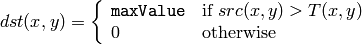
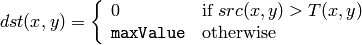
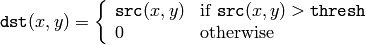
The function transforms a grayscale image to a binary image according to the formulas:
THRESH_BINARY
THRESH_BINARY_INV
where
 is a threshold calculated individually for each pixel.
- For the method
ADAPTIVE_THRESH_MEAN_C
the threshold value
is the mean of a
 neighborhood of
 , minus
C
.
, minus
C
. - For the method
ADAPTIVE_THRESH_GAUSSIAN_C
the threshold value
 is the weighted sum (i.e. cross-correlation with a Gaussian window) of a
neighborhood of
, minus
C
. The default sigma (standard deviation) is used for the specified
blockSize
, see
getGaussianKernel()
.
is the weighted sum (i.e. cross-correlation with a Gaussian window) of a
neighborhood of
, minus
C
. The default sigma (standard deviation) is used for the specified
blockSize
, see
getGaussianKernel()
.
The function can process the image in-place.
See also: threshold() , blur() , GaussianBlur()
cv::cvtColor
- void cvtColor(const Mat& src, Mat& dst, int code, int dstCn=0)
Converts image from one color space to another
Parameters: - src – The source image, 8-bit unsigned, 16-bit unsigned ( CV_16UC... ) or single-precision floating-point
- dst – The destination image; will have the same size and the same depth as src
- code – The color space conversion code; see the discussion
- dstCn – The number of channels in the destination image; if the parameter is 0, the number of the channels will be derived automatically from src and the code
The function converts the input image from one color space to another. In the case of transformation to-from RGB color space the ordering of the channels should be specified explicitly (RGB or BGR).
The conventional ranges for R, G and B channel values are:
- 0 to 255 for CV_8U images
- 0 to 65535 for CV_16U images and
- 0 to 1 for CV_32F images.
Of course, in the case of linear transformations the range does not matter,
but in the non-linear cases the input RGB image should be normalized to the proper value range in order to get the correct results, e.g. for RGB
 L*u*v* transformation. For example, if you have a 32-bit floating-point image directly converted from 8-bit image without any scaling, then it will have 0..255 value range, instead of the assumed by the function 0..1. So, before calling
cvtColor
, you need first to scale the image down:
L*u*v* transformation. For example, if you have a 32-bit floating-point image directly converted from 8-bit image without any scaling, then it will have 0..255 value range, instead of the assumed by the function 0..1. So, before calling
cvtColor
, you need first to scale the image down:
img *= 1./255;
cvtColor(img, img, CV_BGR2Luv);
The function can do the following transformations:
Transformations within RGB space like adding/removing the alpha channel, reversing the channel order, conversion to/from 16-bit RGB color (R5:G6:B5 or R5:G5:B5), as well as conversion to/from grayscale using:
![\text{RGB[A] to Gray:} \quad Y \leftarrow 0.299 \cdot R + 0.587 \cdot G + 0.114 \cdot B](_images/math/aec60f2c1832bb07ad040335189257e97afd00d6.png)
and
![\text{Gray to RGB[A]:} \quad R \leftarrow Y, G \leftarrow Y, B \leftarrow Y, A \leftarrow 0](_images/math/8f5c51f3a4cae34d417208c8f561b2b5e264dc41.png)
The conversion from a RGB image to gray is done with:
cvtColor(src, bwsrc, CV_RGB2GRAY);
Some more advanced channel reordering can also be done with mixChannels() .
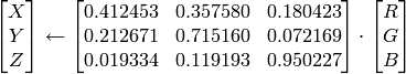
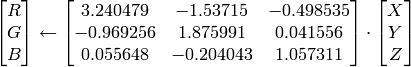
RGB
 CIE XYZ.Rec 709 with D65 white point (
CV_BGR2XYZ, CV_RGB2XYZ, CV_XYZ2BGR, CV_XYZ2RGB
):
CIE XYZ.Rec 709 with D65 white point (
CV_BGR2XYZ, CV_RGB2XYZ, CV_XYZ2BGR, CV_XYZ2RGB
):
 ,
,
 and
and
 cover the whole value range (in the case of floating-point images
may exceed 1).
cover the whole value range (in the case of floating-point images
may exceed 1).RGB
YCrCb JPEG (a.k.a. YCC) (
CV_BGR2YCrCb, CV_RGB2YCrCb, CV_YCrCb2BGR, CV_YCrCb2RGB
)


where
Y, Cr and Cb cover the whole value range.
RGB
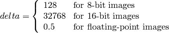
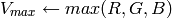
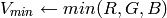
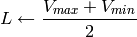
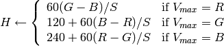
HSV (
CV_BGR2HSV, CV_RGB2HSV, CV_HSV2BGR, CV_HSV2RGB
)in the case of 8-bit and 16-bit images R, G and B are converted to floating-point format and scaled to fit the 0 to 1 range
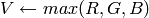
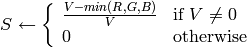
if
 then
then
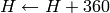 On output
 ,
,
 ,
,
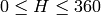 .
.The values are then converted to the destination data type:
8-bit images

16-bit images (currently not supported)

- 32-bit images
H, S, V are left as is
RGB
HLS (
CV_BGR2HLS, CV_RGB2HLS, CV_HLS2BGR, CV_HLS2RGB
).in the case of 8-bit and 16-bit images R, G and B are converted to floating-point format and scaled to fit the 0 to 1 range.
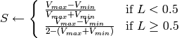
if
then
On output
 ,
,
.
,
,
.The values are then converted to the destination data type:
8-bit images

16-bit images (currently not supported)

- 32-bit images
H, S, V are left as is
RGB
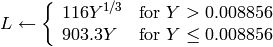
CIE L*a*b* (
CV_BGR2Lab, CV_RGB2Lab, CV_Lab2BGR, CV_Lab2RGB
)in the case of 8-bit and 16-bit images R, G and B are converted to floating-point format and scaled to fit the 0 to 1 range


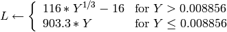


where
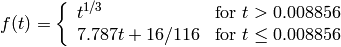
and
On output
 ,
,
 ,
,
 The values are then converted to the destination data type:
8-bit images

- 16-bit images
currently not supported
- 32-bit images
L, a, b are left as is
RGB
CIE L*u*v* (
CV_BGR2Luv, CV_RGB2Luv, CV_Luv2BGR, CV_Luv2RGB
)in the case of 8-bit and 16-bit images R, G and B are converted to floating-point format and scaled to fit 0 to 1 range


On output
,
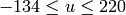 ,
,
 .
.The values are then converted to the destination data type:
8-bit images

- 16-bit images
currently not supported
- 32-bit images
L, u, v are left as is
The above formulas for converting RGB to/from various color spaces have been taken from multiple sources on Web, primarily from the Charles Poynton site http://www.poynton.com/ColorFAQ.html
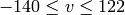
Bayer
RGB (
CV_BayerBG2BGR, CV_BayerGB2BGR, CV_BayerRG2BGR, CV_BayerGR2BGR, CV_BayerBG2RGB, CV_BayerGB2RGB, CV_BayerRG2RGB, CV_BayerGR2RGB
) The Bayer pattern is widely used in CCD and CMOS cameras. It allows one to get color pictures from a single plane where R,G and B pixels (sensors of a particular component) are interleaved like this: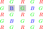
The output RGB components of a pixel are interpolated from 1, 2 or 4 neighbors of the pixel having the same color. There are several modifications of the above pattern that can be achieved by shifting the pattern one pixel left and/or one pixel up. The two letters
 and
and
 in the conversion constants
CV_Bayer
in the conversion constants
CV_Bayer
 2BGR
and
CV_Bayer
2RGB
indicate the particular pattern
type - these are components from the second row, second and third
columns, respectively. For example, the above pattern has very
popular “BG” type.
2BGR
and
CV_Bayer
2RGB
indicate the particular pattern
type - these are components from the second row, second and third
columns, respectively. For example, the above pattern has very
popular “BG” type.
cv::distanceTransform
- void distanceTransform(const Mat& src, Mat& dst, Mat& labels, int distanceType, int maskSize)
Calculates the distance to the closest zero pixel for each pixel of the source image.
Parameters: - src – 8-bit, single-channel (binary) source image
- dst – Output image with calculated distances; will be 32-bit floating-point, single-channel image of the same size as src
- distanceType – Type of distance; can be CV_DIST_L1, CV_DIST_L2 or CV_DIST_C
- maskSize – Size of the distance transform mask; can be 3, 5 or CV_DIST_MASK_PRECISE (the latter option is only supported by the first of the functions). In the case of CV_DIST_L1 or CV_DIST_C distance type the parameter is forced to 3, because a
 mask gives the same result as a
  or any larger aperture.
 - labels – The optional output 2d array of labels - the discrete Voronoi diagram; will have type CV_32SC1 and the same size as src . See the discussion
The functions distanceTransform calculate the approximate or precise distance from every binary image pixel to the nearest zero pixel. (for zero image pixels the distance will obviously be zero).
When maskSize == CV_DIST_MASK_PRECISE and distanceType == CV_DIST_L2 , the function runs the algorithm described in [Felzenszwalb04] .
In other cases the algorithm
[Borgefors86]
is used, that is,
for pixel the function finds the shortest path to the nearest zero pixel
consisting of basic shifts: horizontal,
vertical, diagonal or knight’s move (the latest is available for a
mask). The overall distance is calculated as a sum of these
basic distances. Because the distance function should be symmetric,
all of the horizontal and vertical shifts must have the same cost (that
is denoted as
a
), all the diagonal shifts must have the
same cost (denoted
b
), and all knight’s moves must have
the same cost (denoted
c
). For
CV_DIST_C
and
CV_DIST_L1
types the distance is calculated precisely,
whereas for
CV_DIST_L2
(Euclidian distance) the distance
can be calculated only with some relative error (a
mask
gives more accurate results). For
a
,
b
and
c
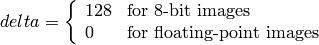
OpenCV uses the values suggested in the original paper:
| CV_DIST_C |  |
a = 1, b = 1 |
|---|---|---|
| CV_DIST_L1 | |
a = 1, b = 2 |
| CV_DIST_L2 | |
a=0.955, b=1.3693 |
| CV_DIST_L2 |  |
a=1, b=1.4, c=2.1969 |
Typically, for a fast, coarse distance estimation
CV_DIST_L2
,
a
mask is used, and for a more accurate distance estimation
CV_DIST_L2
, a
mask or the precise algorithm is used.
Note that both the precise and the approximate algorithms are linear on the number of pixels.
The second variant of the function does not only compute the minimum distance for each pixel
,
but it also identifies the nearest the nearest connected
component consisting of zero pixels. Index of the component is stored in
 .
The connected components of zero pixels are also found and marked by the function.
.
The connected components of zero pixels are also found and marked by the function.
In this mode the complexity is still linear. That is, the function provides a very fast way to compute Voronoi diagram for the binary image. Currently, this second variant can only use the approximate distance transform algorithm.
cv::floodFill
- int floodFill(Mat& image, Point seed, Scalar newVal, Rect* rect=0, Scalar loDiff=Scalar(), Scalar upDiff=Scalar(), int flags=4)
- int floodFill(Mat& image, Mat& mask, Point seed, Scalar newVal, Rect* rect=0, Scalar loDiff=Scalar(), Scalar upDiff=Scalar(), int flags=4)
Fills a connected component with the given color.
Parameters: - image – Input/output 1- or 3-channel, 8-bit or floating-point image. It is modified by the function unless the FLOODFILL_MASK_ONLY flag is set (in the second variant of the function; see below)
- mask – (For the second function only) Operation mask, should be a single-channel 8-bit image, 2 pixels wider and 2 pixels taller. The function uses and updates the mask, so the user takes responsibility of initializing the mask content. Flood-filling can’t go across non-zero pixels in the mask, for example, an edge detector output can be used as a mask to stop filling at edges. It is possible to use the same mask in multiple calls to the function to make sure the filled area do not overlap. Note : because the mask is larger than the filled image, a pixel in image will correspond to the pixel
 in the mask
 - seed – The starting point
- newVal – New value of the repainted domain pixels
- loDiff – Maximal lower brightness/color difference between the currently observed pixel and one of its neighbors belonging to the component, or a seed pixel being added to the component
- upDiff – Maximal upper brightness/color difference between the currently observed pixel and one of its neighbors belonging to the component, or a seed pixel being added to the component
- rect – The optional output parameter that the function sets to the minimum bounding rectangle of the repainted domain
- flags –
The operation flags. Lower bits contain connectivity value, 4 (by default) or 8, used within the function. Connectivity determines which neighbors of a pixel are considered. Upper bits can be 0 or a combination of the following flags:
- FLOODFILL_FIXED_RANGE if set, the difference between the current pixel and seed pixel is considered, otherwise the difference between neighbor pixels is considered (i.e. the range is floating)
- FLOODFILL_MASK_ONLY (for the second variant only) if set, the function does not change the image ( newVal is ignored), but fills the mask
The functions
floodFill
fill a connected component starting from the seed point with the specified color. The connectivity is determined by the color/brightness closeness of the neighbor pixels. The pixel at
 is considered to belong to the repainted domain if:
grayscale image, floating range

grayscale image, fixed range

color image, floating range


color image, fixed range


where
 is the value of one of pixel neighbors that is already known to belong to the component. That is, to be added to the connected component, a pixel’s color/brightness should be close enough to the:
- color/brightness of one of its neighbors that are already referred to the connected component in the case of floating range
- color/brightness of the seed point in the case of fixed range.
By using these functions you can either mark a connected component with the specified color in-place, or build a mask and then extract the contour or copy the region to another image etc. Various modes of the function are demonstrated in floodfill.c sample.
See also: findContours()
cv::inpaint
- void inpaint(const Mat& src, const Mat& inpaintMask, Mat& dst, double inpaintRadius, int flags)
Inpaints the selected region in the image.
Parameters: - src – The input 8-bit 1-channel or 3-channel image.
- inpaintMask – The inpainting mask, 8-bit 1-channel image. Non-zero pixels indicate the area that needs to be inpainted.
- dst – The output image; will have the same size and the same type as src
- inpaintRadius – The radius of a circlular neighborhood of each point inpainted that is considered by the algorithm.
- flags –
The inpainting method, one of the following:
- INPAINT_NS Navier-Stokes based method.
- INPAINT_TELEA The method by Alexandru Telea [Telea04]
The function reconstructs the selected image area from the pixel near the area boundary. The function may be used to remove dust and scratches from a scanned photo, or to remove undesirable objects from still images or video. See http://en.wikipedia.org/wiki/Inpainting for more details.
cv::integral
- void integral(const Mat& image, Mat& sum, Mat& sqsum, Mat& tilted, int sdepth=-1)
Calculates the integral of an image.
Parameters: - image – The source image,
 , 8-bit or floating-point (32f or 64f)
 - sum – The integral image,
 , 32-bit integer or floating-point (32f or 64f)
 - sqsum – The integral image for squared pixel values, , double precision floating-point (64f)
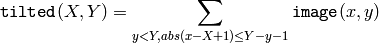
- tilted – The integral for the image rotated by 45 degrees, , the same data type as sum
- sdepth – The desired depth of the integral and the tilted integral images, CV_32S , CV_32F or CV_64F
- image – The source image,
The functions integral calculate one or more integral images for the source image as following:
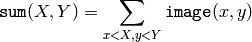
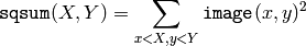
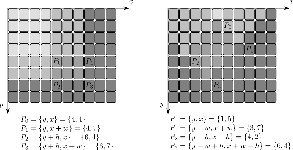
Using these integral images, one may calculate sum, mean and standard deviation over a specific up-right or rotated rectangular region of the image in a constant time, for example:

It makes possible to do a fast blurring or fast block correlation with variable window size, for example. In the case of multi-channel images, sums for each channel are accumulated independently.
As a practical example, the next figure shows the calculation of the integral of a straight rectangle Rect(3,3,3,2) and of a tilted rectangle Rect(5,1,2,3) . The selected pixels in the original image are shown, as well as the relative pixels in the integral images sum and tilted .
begin{center}
end{center}
cv::threshold
- double threshold(const Mat& src, Mat& dst, double thresh, double maxVal, int thresholdType)
Applies a fixed-level threshold to each array element
Parameters: - src – Source array (single-channel, 8-bit of 32-bit floating point)
- dst – Destination array; will have the same size and the same type as src
- thresh – Threshold value
- maxVal – Maximum value to use with THRESH_BINARY and THRESH_BINARY_INV thresholding types
- thresholdType – Thresholding type (see the discussion)
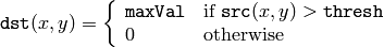
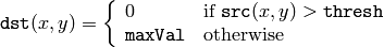
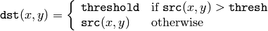
The function applies fixed-level thresholding to a single-channel array. The function is typically used to get a bi-level (binary) image out of a grayscale image ( compare() could be also used for this purpose) or for removing a noise, i.e. filtering out pixels with too small or too large values. There are several types of thresholding that the function supports that are determined by thresholdType :
THRESH_BINARY
THRESH_BINARY_INV
THRESH_TRUNC
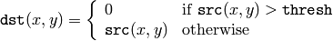
THRESH_TOZERO
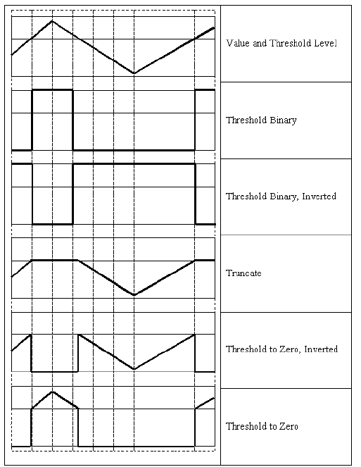
THRESH_TOZERO_INV
Also, the special value THRESH_OTSU may be combined with one of the above values. In this case the function determines the optimal threshold value using Otsu’s algorithm and uses it instead of the specified thresh . The function returns the computed threshold value. Currently, Otsu’s method is implemented only for 8-bit images.
See also: adaptiveThreshold() , findContours() , compare() , min() , max()
cv::watershed
- void watershed(const Mat& image, Mat& markers)
Does marker-based image segmentation using watershed algrorithm
Parameters: - image – The input 8-bit 3-channel image.
- markers – The input/output 32-bit single-channel image (map) of markers. It should have the same size as image
The function implements one of the variants
of watershed, non-parametric marker-based segmentation algorithm,
described in
[Meyer92]
. Before passing the image to the
function, user has to outline roughly the desired regions in the image
markers
with positive (
 ) indices, i.e. every region is
represented as one or more connected components with the pixel values
1, 2, 3 etc (such markers can be retrieved from a binary mask
using
findContours()
and
drawContours()
, see
watershed.cpp
demo).
The markers will be “seeds” of the future image
regions. All the other pixels in
markers
, which relation to the
outlined regions is not known and should be defined by the algorithm,
should be set to 0’s. On the output of the function, each pixel in
markers is set to one of values of the “seed” components, or to -1 at
boundaries between the regions.
) indices, i.e. every region is
represented as one or more connected components with the pixel values
1, 2, 3 etc (such markers can be retrieved from a binary mask
using
findContours()
and
drawContours()
, see
watershed.cpp
demo).
The markers will be “seeds” of the future image
regions. All the other pixels in
markers
, which relation to the
outlined regions is not known and should be defined by the algorithm,
should be set to 0’s. On the output of the function, each pixel in
markers is set to one of values of the “seed” components, or to -1 at
boundaries between the regions.
Note, that it is not necessary that every two neighbor connected components are separated by a watershed boundary (-1’s pixels), for example, in case when such tangent components exist in the initial marker image. Visual demonstration and usage example of the function can be found in OpenCV samples directory; see watershed.cpp demo.
See also: findContours()
Help and Feedback
You did not find what you were looking for?- Try the FAQ.
- Ask a question in the user group/mailing list.
- If you think something is missing or wrong in the documentation, please file a bug report.