Structural Analysis and Shape Descriptors
cv::moments
- Moments moments(const Mat& array, bool binaryImage=false)
Calculates all of the moments up to the third order of a polygon or rasterized shape.
where the class Moments is defined as:
class Moments
{
public:
    Moments();
    Moments(double m00, double m10, double m01, double m20, double m11,
            double m02, double m30, double m21, double m12, double m03 );
    Moments( const CvMoments& moments );
    operator CvMoments() const;

    // spatial moments
    double  m00, m10, m01, m20, m11, m02, m30, m21, m12, m03;
    // central moments
    double  mu20, mu11, mu02, mu30, mu21, mu12, mu03;
    // central normalized moments
    double  nu20, nu11, nu02, nu30, nu21, nu12, nu03;
};
param array: A raster image (single-channel, 8-bit or floating-point 2D array) or an array ( or
) of 2D points ( Point or Point2f )
param binaryImage: (For images only) If it is true, then all the non-zero image pixels are treated as 1’s
The function computes moments, up to the 3rd order, of a vector shape or a rasterized shape.
In case of a raster image, the spatial moments
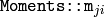 are computed as:
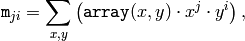
the central moments
 are computed as:
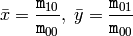
where
 is the mass center:
and the normalized central moments
 are computed as:
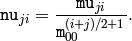
Note that
 ,
,

 , hence the values are not stored.
The moments of a contour are defined in the same way, but computed using Green’s formula (see http://en.wikipedia.org/wiki/Green_theorem ), therefore, because of a limited raster resolution, the moments computed for a contour will be slightly different from the moments computed for the same contour rasterized.
See also: contourArea() , arcLength()
cv::HuMoments
- void HuMoments(const Moments& moments, double h[7])
Calculates the seven Hu invariants.
Parameters: - moments – The input moments, computed with moments()
- h – The output Hu invariants
The function calculates the seven Hu invariants, see http://en.wikipedia.org/wiki/Image_moment , that are defined as:
![\begin{array}{l} h[0]= \eta _{20}+ \eta _{02} \\ h[1]=( \eta _{20}- \eta _{02})^{2}+4 \eta _{11}^{2} \\ h[2]=( \eta _{30}-3 \eta _{12})^{2}+ (3 \eta _{21}- \eta _{03})^{2} \\ h[3]=( \eta _{30}+ \eta _{12})^{2}+ ( \eta _{21}+ \eta _{03})^{2} \\ h[4]=( \eta _{30}-3 \eta _{12})( \eta _{30}+ \eta _{12})[( \eta _{30}+ \eta _{12})^{2}-3( \eta _{21}+ \eta _{03})^{2}]+(3 \eta _{21}- \eta _{03})( \eta _{21}+ \eta _{03})[3( \eta _{30}+ \eta _{12})^{2}-( \eta _{21}+ \eta _{03})^{2}] \\ h[5]=( \eta _{20}- \eta _{02})[( \eta _{30}+ \eta _{12})^{2}- ( \eta _{21}+ \eta _{03})^{2}]+4 \eta _{11}( \eta _{30}+ \eta _{12})( \eta _{21}+ \eta _{03}) \\ h[6]=(3 \eta _{21}- \eta _{03})( \eta _{21}+ \eta _{03})[3( \eta _{30}+ \eta _{12})^{2}-( \eta _{21}+ \eta _{03})^{2}]-( \eta _{30}-3 \eta _{12})( \eta _{21}+ \eta _{03})[3( \eta _{30}+ \eta _{12})^{2}-( \eta _{21}+ \eta _{03})^{2}] \\ \end{array}](_images/math/8abf2554aad5cce3dd3291abe515b3a8dcc3a1bd.png)
where
 stand for
 .
.
These values are proved to be invariant to the image scale, rotation, and reflection except the seventh one, whose sign is changed by reflection. Of course, this invariance was proved with the assumption of infinite image resolution. In case of a raster images the computed Hu invariants for the original and transformed images will be a bit different.
See also: matchShapes()
cv::findContours
- void findContours(const Mat& image, vector<vector<Point> >& contours, vector<Vec4i>& hierarchy, int mode, int method, Point offset=Point())
- void findContours(const Mat& image, vector<vector<Point> >& contours, int mode, int method, Point offset=Point())
Finds the contours in a binary image.
Parameters: - image – The source, an 8-bit single-channel image. Non-zero pixels are treated as 1’s, zero pixels remain 0’s - the image is treated as binary . You can use compare() , inRange() , threshold() , adaptiveThreshold() , Canny() etc. to create a binary image out of a grayscale or color one. The function modifies the image while extracting the contours
- contours – The detected contours. Each contour is stored as a vector of points
- hiararchy – The optional output vector that will contain information about the image topology. It will have as many elements as the number of contours. For each contour contours[i] , the elements hierarchy[i][0] , hiearchy[i][1] , hiearchy[i][2] , hiearchy[i][3] will be set to 0-based indices in contours of the next and previous contours at the same hierarchical level, the first child contour and the parent contour, respectively. If for some contour i there is no next, previous, parent or nested contours, the corresponding elements of hierarchy[i] will be negative
- mode –
The contour retrieval mode
- CV_RETR_EXTERNAL retrieves only the extreme outer contours; It will set hierarchy[i][2]=hierarchy[i][3]=-1 for all the contours
- CV_RETR_LIST retrieves all of the contours without establishing any hierarchical relationships
- CV_RETR_CCOMP retrieves all of the contours and organizes them into a two-level hierarchy: on the top level are the external boundaries of the components, on the second level are the boundaries of the holes. If inside a hole of a connected component there is another contour, it will still be put on the top level
- CV_RETR_TREE retrieves all of the contours and reconstructs the full hierarchy of nested contours. This full hierarchy is built and shown in OpenCV contours.c demo
- method –
The contour approximation method.
- CV_CHAIN_APPROX_NONE stores absolutely all the contour points. That is, every 2 points of a contour stored with this method are 8-connected neighbors of each other
- CV_CHAIN_APPROX_SIMPLE compresses horizontal, vertical, and diagonal segments and leaves only their end points. E.g. an up-right rectangular contour will be encoded with 4 points
- CV_CHAIN_APPROX_TC89_L1,CV_CHAIN_APPROX_TC89_KCOS applies one of the flavors of the Teh-Chin chain approximation algorithm; see TehChin89
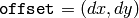
- offset – The optional offset, by which every contour point is shifted. This is useful if the contours are extracted from the image ROI and then they should be analyzed in the whole image context
The function retrieves contours from the binary image using the algorithm Suzuki85 . The contours are a useful tool for shape analysis and object detection and recognition. See squares.c in the OpenCV sample directory.
Note: the source image is modified by this function.
cv::drawContours
- void drawContours(Mat& image, const vector<vector<Point> >& contours, int contourIdx, const Scalar& color, int thickness=1, int lineType=8, const vector<Vec4i>& hierarchy=vector<Vec4i>(), int maxLevel=INT_MAX, Point offset=Point())
Draws contours’ outlines or filled contours.
Parameters: - image – The destination image
- contours – All the input contours. Each contour is stored as a point vector
- contourIdx – Indicates the contour to draw. If it is negative, all the contours are drawn
- color – The contours’ color
- thickness – Thickness of lines the contours are drawn with. If it is negative (e.g. thickness=CV_FILLED ), the contour interiors are drawn.
- lineType – The line connectivity; see line() description
- hierarchy – The optional information about hierarchy. It is only needed if you want to draw only some of the contours (see maxLevel )
- maxLevel – Maximal level for drawn contours. If 0, only the specified contour is drawn. If 1, the function draws the contour(s) and all the nested contours. If 2, the function draws the contours, all the nested contours and all the nested into nested contours etc. This parameter is only taken into account when there is hierarchy available.
- offset – The optional contour shift parameter. Shift all the drawn contours by the specified
The function draws contour outlines in the image if
 or fills the area bounded by the contours if
 . Here is the example on how to retrieve connected components from the binary image and label them
#include "cv.h"
#include "highgui.h"

using namespace cv;

int main( int argc, char** argv )
{
    Mat src;
    // the first command line parameter must be file name of binary
    // (black-n-white) image
    if( argc != 2 || !(src=imread(argv[1], 0)).data)
        return -1;

    Mat dst = Mat::zeros(src.rows, src.cols, CV_8UC3);

    src = src > 1;
    namedWindow( "Source", 1 );
    imshow( "Source", src );

    vector<vector<Point> > contours;
    vector<Vec4i> hierarchy;

    findContours( src, contours, hierarchy,
        CV_RETR_CCOMP, CV_CHAIN_APPROX_SIMPLE );

    // iterate through all the top-level contours,
    // draw each connected component with its own random color
    int idx = 0;
    for( ; idx >= 0; idx = hierarchy[idx][0] )
    {
        Scalar color( rand()&255, rand()&255, rand()&255 );
        drawContours( dst, contours, idx, color, CV_FILLED, 8, hierarchy );
    }

    namedWindow( "Components", 1 );
    imshow( "Components", dst );
    waitKey(0);
}
cv::approxPolyDP
- void approxPolyDP(const Mat& curve, vector<Point2f>& approxCurve, double epsilon, bool closed)
Approximates polygonal curve(s) with the specified precision.
Parameters: - curve – The polygon or curve to approximate. Must be or matrix of type CV_32SC2 or CV_32FC2 . You can also convert vector<Point> or vector<Point2f to the matrix by calling Mat(const vector<T>&) constructor.
- approxCurve – The result of the approximation; The type should match the type of the input curve
- epsilon – Specifies the approximation accuracy. This is the maximum distance between the original curve and its approximation
- closed – If true, the approximated curve is closed (i.e. its first and last vertices are connected), otherwise it’s not
- curve – The polygon or curve to approximate. Must be
The functions approxPolyDP approximate a curve or a polygon with another curve/polygon with less vertices, so that the distance between them is less or equal to the specified precision. It used Douglas-Peucker algorithm http://en.wikipedia.org/wiki/Ramer-Douglas-Peucker_algorithm
cv::arcLength
- double arcLength(const Mat& curve, bool closed)
Calculates a contour perimeter or a curve length.
Parameters: - curve – The input vector of 2D points, represented by CV_32SC2 or CV_32FC2 matrix, or by vector<Point> or vector<Point2f> converted to a matrix with Mat(const vector<T>&) constructor
- closed – Indicates, whether the curve is closed or not
The function computes the curve length or the closed contour perimeter.
cv::boundingRect
- Rect boundingRect(const Mat& points)
Calculates the up-right bounding rectangle of a point set.
Parameters: - points – The input 2D point set, represented by CV_32SC2 or CV_32FC2 matrix, or by vector<Point> or vector<Point2f> converted to the matrix using Mat(const vector<T>&) constructor.
The function calculates and returns the minimal up-right bounding rectangle for the specified point set.
cv::estimateRigidTransform
- Mat estimateRigidTransform(const Mat& srcpt, const Mat& dstpt, bool fullAffine)
Computes optimal affine transformation between two 2D point sets
Parameters: - srcpt – The first input 2D point set
- dst – The second input 2D point set of the same size and the same type as A
- fullAffine – If true, the function finds the optimal affine transformation with no any additional resrictions (i.e. there are 6 degrees of freedom); otherwise, the class of transformations to choose from is limited to combinations of translation, rotation and uniform scaling (i.e. there are 5 degrees of freedom)
The function finds the optimal affine transform
![[A|b]](_images/math/5811dc4a2ff4e426ab272d1d4da6988db5790e51.png) (a
(a
 floating-point matrix) that approximates best the transformation from
 to
to
 :
:
![[A^*|b^*] = arg \min _{[A|b]} \sum _i \| \texttt{dstpt} _i - A { \texttt{srcpt} _i}^T - b \| ^2](_images/math/4cb9f8958a90e9902498766c05c0f252459343d1.png)
where
can be either arbitrary (when
fullAffine=true
) or have form
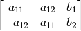
when fullAffine=false .
See also: getAffineTransform() , getPerspectiveTransform() , findHomography()
cv::estimateAffine3D
- int estimateAffine3D(const Mat& srcpt, const Mat& dstpt, Mat& out, vector<uchar>& outliers, double ransacThreshold = 3.0, double confidence = 0.99)
Computes optimal affine transformation between two 3D point sets
Parameters: - srcpt – The first input 3D point set
- dstpt – The second input 3D point set
- out – The output 3D affine transformation matrix

- outliers – The output vector indicating which points are outliers
- ransacThreshold – The maximum reprojection error in RANSAC algorithm to consider a point an inlier
- confidence – The confidence level, between 0 and 1, with which the matrix is estimated
The function estimates the optimal 3D affine transformation between two 3D point sets using RANSAC algorithm.
cv::contourArea
- double contourArea(const Mat& contour)
Calculates the contour area
Parameters: - contour – The contour vertices, represented by CV_32SC2 or CV_32FC2 matrix, or by vector<Point> or vector<Point2f> converted to the matrix using Mat(const vector<T>&) constructor.
The function computes the contour area. Similarly to moments() the area is computed using the Green formula, thus the returned area and the number of non-zero pixels, if you draw the contour using drawContours() or fillPoly() , can be different. Here is a short example:
vector<Point> contour;
contour.push_back(Point2f(0, 0));
contour.push_back(Point2f(10, 0));
contour.push_back(Point2f(10, 10));
contour.push_back(Point2f(5, 4));

double area0 = contourArea(contour);
vector<Point> approx;
approxPolyDP(contour, approx, 5, true);
double area1 = contourArea(approx);

cout << "area0 =" << area0 << endl <<
        "area1 =" << area1 << endl <<
        "approx poly vertices" << approx.size() << endl;
cv::convexHull
- void convexHull(const Mat& points, vector<Point>& hull, bool clockwise=false)
- void convexHull(const Mat& points, vector<Point2f>& hull, bool clockwise=false)
Finds the convex hull of a point set.
Parameters: - points – The input 2D point set, represented by CV_32SC2 or CV_32FC2 matrix, or by vector<Point> or vector<Point2f> converted to the matrix using Mat(const vector<T>&) constructor.
- hull – The output convex hull. It is either a vector of points that form the hull (must have the same type as the input points), or a vector of 0-based point indices of the hull points in the original array (since the set of convex hull points is a subset of the original point set).
- clockwise – If true, the output convex hull will be oriented clockwise, otherwise it will be oriented counter-clockwise. Here, the usual screen coordinate system is assumed - the origin is at the top-left corner, x axis is oriented to the right, and y axis is oriented downwards.
The functions find the convex hull of a 2D point set using Sklansky’s algorithm
Sklansky82
that has
 or
or
 complexity (where
 is the number of input points), depending on how the initial sorting is implemented (currently it is
. See the OpenCV sample
convexhull.c
that demonstrates the use of the different function variants.
is the number of input points), depending on how the initial sorting is implemented (currently it is
. See the OpenCV sample
convexhull.c
that demonstrates the use of the different function variants.
cv::fitEllipse
- RotatedRect fitEllipse(const Mat& points)
Fits an ellipse around a set of 2D points.
Parameters: - points – The input 2D point set, represented by CV_32SC2 or CV_32FC2 matrix, or by vector<Point> or vector<Point2f> converted to the matrix using Mat(const vector<T>&) constructor.
The function calculates the ellipse that fits best (in least-squares sense) a set of 2D points. It returns the rotated rectangle in which the ellipse is inscribed.
cv::fitLine
- void fitLine(const Mat& points, Vec6f& line, int distType, double param, double reps, double aeps)
Fits a line to a 2D or 3D point set.
Parameters: - points – The input 2D point set, represented by CV_32SC2 or CV_32FC2 matrix, or by vector<Point> , vector<Point2f> , vector<Point3i> or vector<Point3f> converted to the matrix by Mat(const vector<T>&) constructor
- line –
The output line parameters. In the case of a 2d fitting, it is a vector of 4 floats ``(vx, vy,
x0, y0)`` where (vx, vy) is a normalized vector collinear to the
line and (x0, y0) is some point on the line. in the case of a 3D fitting it is vector of 6 floats (vx, vy, vz, x0, y0, z0) where (vx, vy, vz) is a normalized vector collinear to the line and (x0, y0, z0) is some point on the line
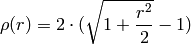
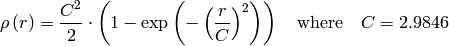
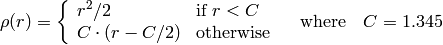
- distType – The distance used by the M-estimator (see the discussion)
- param – Numerical parameter ( C ) for some types of distances, if 0 then some optimal value is chosen
- aeps (reps,) – Sufficient accuracy for the radius (distance between the coordinate origin and the line) and angle, respectively; 0.01 would be a good default value for both.
The functions
fitLine
fit a line to a 2D or 3D point set by minimizing
 where
where
 is the distance between the
 point and the line and
 is a distance function, one of:
distType=CV_DIST_L2

distType=CV_DIST_L1

distType=CV_DIST_L12
distType=CV_DIST_FAIR

distType=CV_DIST_WELSCH
distType=CV_DIST_HUBER
The algorithm is based on the M-estimator (
http://en.wikipedia.org/wiki/M-estimator
) technique, that iteratively fits the line using weighted least-squares algorithm and after each iteration the weights
 are adjusted to beinversely proportional to
 .
.
cv::isContourConvex
- bool isContourConvex(const Mat& contour)
Tests contour convexity.
Parameters: - contour – The tested contour, a matrix of type CV_32SC2 or CV_32FC2 , or vector<Point> or vector<Point2f> converted to the matrix using Mat(const vector<T>&) constructor.
The function tests whether the input contour is convex or not. The contour must be simple, i.e. without self-intersections, otherwise the function output is undefined.
cv::minAreaRect
- RotatedRect minAreaRect(const Mat& points)
Finds the minimum area rotated rectangle enclosing a 2D point set.
Parameters: - points – The input 2D point set, represented by CV_32SC2 or CV_32FC2 matrix, or by vector<Point> or vector<Point2f> converted to the matrix using Mat(const vector<T>&) constructor.
The function calculates and returns the minimum area bounding rectangle (possibly rotated) for the specified point set. See the OpenCV sample minarea.c
cv::minEnclosingCircle
- void minEnclosingCircle(const Mat& points, Point2f& center, float& radius)
Finds the minimum area circle enclosing a 2D point set.
Parameters: - points – The input 2D point set, represented by CV_32SC2 or CV_32FC2 matrix, or by vector<Point> or vector<Point2f> converted to the matrix using Mat(const vector<T>&) constructor.
- center – The output center of the circle
- radius – The output radius of the circle
The function finds the minimal enclosing circle of a 2D point set using iterative algorithm. See the OpenCV sample minarea.c
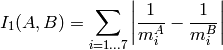
cv::matchShapes
- double matchShapes(const Mat& object1, const Mat& object2, int method, double parameter=0)
Compares two shapes.
Parameters: - object1 – The first contour or grayscale image
- object2 – The second contour or grayscale image
- method –
- Comparison method:
- CV_CONTOUR_MATCH_I1 , CV_CONTOURS_MATCH_I2
- or
- CV_CONTOURS_MATCH_I3 (see the discussion below)
- parameter – Method-specific parameter (is not used now)
The function compares two shapes. The 3 implemented methods all use Hu invariants (see
HuMoments()
) as following (
 denotes
object1
,
denotes
object1
,
 denotes
object2
):
denotes
object2
):
method=CV_CONTOUR_MATCH_I1
method=CV_CONTOUR_MATCH_I2
method=CV_CONTOUR_MATCH_I3
where
and
 are the Hu moments of
and
respectively.
are the Hu moments of
and
respectively.
cv::pointPolygonTest
- double pointPolygonTest(const Mat& contour, Point2f pt, bool measureDist)
Performs point-in-contour test.
Parameters: - contour – The input contour
- pt – The point tested against the contour
- measureDist – If true, the function estimates the signed distance from the point to the nearest contour edge; otherwise, the function only checks if the point is inside or not.
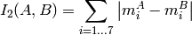
The function determines whether the point is inside a contour, outside, or lies on an edge (or coincides with a vertex). It returns positive (inside), negative (outside) or zero (on an edge) value, correspondingly. When measureDist=false , the return value is +1, -1 and 0, respectively. Otherwise, the return value it is a signed distance between the point and the nearest contour edge.
Here is the sample output of the function, where each image pixel is tested against the contour.
Help and Feedback
You did not find what you were looking for?- Try the Cheatsheet.
- Ask a question in the user group/mailing list.
- If you think something is missing or wrong in the documentation, please file a bug report.
![]()
Table Of Contents
- Structural Analysis and Shape Descriptors
- cv::moments
- cv::HuMoments
- cv::findContours
- cv::drawContours
- cv::approxPolyDP
- cv::arcLength
- cv::boundingRect
- cv::estimateRigidTransform
- cv::estimateAffine3D
- cv::contourArea
- cv::convexHull
- cv::fitEllipse
- cv::fitLine
- cv::isContourConvex
- cv::minAreaRect
- cv::minEnclosingCircle
- cv::matchShapes
- cv::pointPolygonTest
Previous topic
Miscellaneous Image Transformations