Miscellaneous Image Transformations
AdaptiveThreshold
- AdaptiveThreshold(src, dst, maxValue, adaptive_method=CV_ADAPTIVE_THRESH_MEAN_C, thresholdType=CV_THRESH_BINARY, blockSize=3, param1=5) → None
Applies an adaptive threshold to an array.
Parameters: - src (CvArr) – Source image
- dst (CvArr) – Destination image
- maxValue (float) – Maximum value that is used with CV_THRESH_BINARY and CV_THRESH_BINARY_INV
- adaptive_method (int) – Adaptive thresholding algorithm to use: CV_ADAPTIVE_THRESH_MEAN_C or CV_ADAPTIVE_THRESH_GAUSSIAN_C (see the discussion)
- thresholdType (int) –
Thresholding type; must be one of
- CV_THRESH_BINARY xxx
- CV_THRESH_BINARY_INV xxx
- blockSize (int) – The size of a pixel neighborhood that is used to calculate a threshold value for the pixel: 3, 5, 7, and so on
- param1 (float) – The method-dependent parameter. For the methods CV_ADAPTIVE_THRESH_MEAN_C and CV_ADAPTIVE_THRESH_GAUSSIAN_C it is a constant subtracted from the mean or weighted mean (see the discussion), though it may be negative
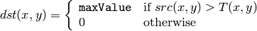
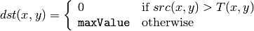
The function transforms a grayscale image to a binary image according to the formulas:
CV_THRESH_BINARY
CV_THRESH_BINARY_INV
where
 is a threshold calculated individually for each pixel.
For the method
CV_ADAPTIVE_THRESH_MEAN_C
it is the mean of a
 pixel neighborhood, minus
param1
.
pixel neighborhood, minus
param1
.
For the method
CV_ADAPTIVE_THRESH_GAUSSIAN_C
it is the weighted sum (gaussian) of a
pixel neighborhood, minus
param1
.
CvtColor
- CvtColor(src, dst, code) → None
Converts an image from one color space to another.
Parameters: - src (CvArr) – The source 8-bit (8u), 16-bit (16u) or single-precision floating-point (32f) image
- dst (CvArr) – The destination image of the same data type as the source. The number of channels may be different
- code (int) – Color conversion operation that can be specifed using CV_ *src_color_space* 2 *dst_color_space* constants (see below)
The function converts the input image from one color
space to another. The function ignores the
colorModel
and
channelSeq
fields of the
IplImage
header, so the
source image color space should be specified correctly (including
order of the channels in the case of RGB space. For example, BGR means 24-bit
format with
 layout
whereas RGB means 24-format with
layout
whereas RGB means 24-format with
 layout).
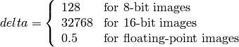
The conventional range for R,G,B channel values is:
- 0 to 255 for 8-bit images
- 0 to 65535 for 16-bit images and
- 0 to 1 for floating-point images.
Of course, in the case of linear transformations the range can be specific, but in order to get correct results in the case of non-linear transformations, the input image should be scaled.
The function can do the following transformations:
Transformations within RGB space like adding/removing the alpha channel, reversing the channel order, conversion to/from 16-bit RGB color (R5:G6:B5 or R5:G5:B5), as well as conversion to/from grayscale using:
![\text{RGB[A] to Gray:} Y \leftarrow 0.299 \cdot R + 0.587 \cdot G + 0.114 \cdot B](_images/math/7424f873dd6b0ad2126a58f9300a2af49c8641a8.png)
and
![\text{Gray to RGB[A]:} R \leftarrow Y, G \leftarrow Y, B \leftarrow Y, A \leftarrow 0](_images/math/b53be450756cbea9860e3518c562fb3c263828de.png)
The conversion from a RGB image to gray is done with:
cvCvtColor(src ,bwsrc, CV_RGB2GRAY)
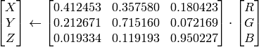
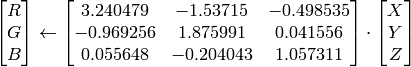
RGB
 CIE XYZ.Rec 709 with D65 white point (
CV_BGR2XYZ, CV_RGB2XYZ, CV_XYZ2BGR, CV_XYZ2RGB
):
CIE XYZ.Rec 709 with D65 white point (
CV_BGR2XYZ, CV_RGB2XYZ, CV_XYZ2BGR, CV_XYZ2RGB
):
 ,
,
 and
and
 cover the whole value range (in the case of floating-point images
may exceed 1).
cover the whole value range (in the case of floating-point images
may exceed 1).RGB
YCrCb JPEG (a.k.a. YCC) (
CV_BGR2YCrCb, CV_RGB2YCrCb, CV_YCrCb2BGR, CV_YCrCb2RGB
)


where
Y, Cr and Cb cover the whole value range.
RGB
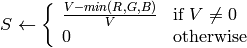
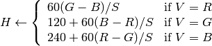
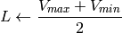
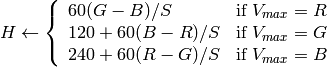
HSV (
CV_BGR2HSV, CV_RGB2HSV, CV_HSV2BGR, CV_HSV2RGB
)
in the case of 8-bit and 16-bit images
R, G and B are converted to floating-point format and scaled to fit the 0 to 1 range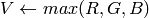
if
 then
then
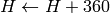 On output
 ,
,
 ,
,
 .
.The values are then converted to the destination data type:
8-bit images

16-bit images (currently not supported)

- 32-bit images
H, S, V are left as is
RGB
HLS (
CV_BGR2HLS, CV_RGB2HLS, CV_HLS2BGR, CV_HLS2RGB
).
in the case of 8-bit and 16-bit images
R, G and B are converted to floating-point format and scaled to fit the 0 to 1 range.
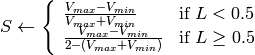
if
then
On output
 ,
,
.
,
,
.The values are then converted to the destination data type:
8-bit images
16-bit images (currently not supported)
- 32-bit images
H, S, V are left as is
RGB
CIE L*a*b* (
CV_BGR2Lab, CV_RGB2Lab, CV_Lab2BGR, CV_Lab2RGB
)
in the case of 8-bit and 16-bit images
R, G and B are converted to floating-point format and scaled to fit the 0 to 1 range


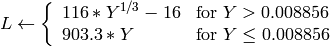


where
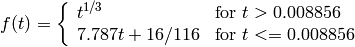
and
On output
 ,
,
 ,
,
 The values are then converted to the destination data type:
8-bit images

- 16-bit images
currently not supported
- 32-bit images
L, a, b are left as is
RGB
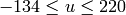
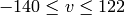
CIE L*u*v* (
CV_BGR2Luv, CV_RGB2Luv, CV_Luv2BGR, CV_Luv2RGB
)
in the case of 8-bit and 16-bit images
R, G and B are converted to floating-point format and scaled to fit 0 to 1 range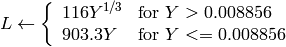


On output
,
 ,
,
 .
.The values are then converted to the destination data type:
8-bit images

- 16-bit images
currently not supported
- 32-bit images
L, u, v are left as is
The above formulas for converting RGB to/from various color spaces have been taken from multiple sources on Web, primarily from the Ford98 at the Charles Poynton site.
Bayer
 RGB (
CV_BayerBG2BGR, CV_BayerGB2BGR, CV_BayerRG2BGR, CV_BayerGR2BGR, CV_BayerBG2RGB, CV_BayerGB2RGB, CV_BayerRG2RGB, CV_BayerGR2RGB
) The Bayer pattern is widely used in CCD and CMOS cameras. It allows one to get color pictures from a single plane where R,G and B pixels (sensors of a particular component) are interleaved like this:
RGB (
CV_BayerBG2BGR, CV_BayerGB2BGR, CV_BayerRG2BGR, CV_BayerGR2BGR, CV_BayerBG2RGB, CV_BayerGB2RGB, CV_BayerRG2RGB, CV_BayerGR2RGB
) The Bayer pattern is widely used in CCD and CMOS cameras. It allows one to get color pictures from a single plane where R,G and B pixels (sensors of a particular component) are interleaved like this: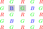
The output RGB components of a pixel are interpolated from 1, 2 or 4 neighbors of the pixel having the same color. There are several modifications of the above pattern that can be achieved by shifting the pattern one pixel left and/or one pixel up. The two letters
 and
and
 in the conversion constants
CV_Bayer
in the conversion constants
CV_Bayer
 2BGR
and
CV_Bayer
2RGB
indicate the particular pattern
type - these are components from the second row, second and third
columns, respectively. For example, the above pattern has very
popular “BG” type.
2BGR
and
CV_Bayer
2RGB
indicate the particular pattern
type - these are components from the second row, second and third
columns, respectively. For example, the above pattern has very
popular “BG” type.
DistTransform
- DistTransform(src, dst, distance_type=CV_DIST_L2, mask_size=3, mask=None, labels=NULL) → None
Calculates the distance to the closest zero pixel for all non-zero pixels of the source image.
Parameters: - src (CvArr) – 8-bit, single-channel (binary) source image
- dst (CvArr) – Output image with calculated distances (32-bit floating-point, single-channel)
- distance_type (int) – Type of distance; can be CV_DIST_L1, CV_DIST_L2, CV_DIST_C or CV_DIST_USER
- mask_size (int) – Size of the distance transform mask; can be 3 or 5. in the case of CV_DIST_L1 or CV_DIST_C the parameter is forced to 3, because a
 mask gives the same result as a
  yet it is faster
 - mask (sequence of float) – User-defined mask in the case of a user-defined distance, it consists of 2 numbers (horizontal/vertical shift cost, diagonal shift cost) in the case ofa mask and 3 numbers (horizontal/vertical shift cost, diagonal shift cost, knight’s move cost) in the case of a mask
- labels (CvArr) – The optional output 2d array of integer type labels, the same size as src and dst
The function calculates the approximated
distance from every binary image pixel to the nearest zero pixel.
For zero pixels the function sets the zero distance, for others it
finds the shortest path consisting of basic shifts: horizontal,
vertical, diagonal or knight’s move (the latest is available for a
mask). The overall distance is calculated as a sum of these
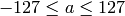
basic distances. Because the distance function should be symmetric,
all of the horizontal and vertical shifts must have the same cost (that
is denoted as
a
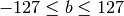
), all the diagonal shifts must have the
same cost (denoted
b
), and all knight’s moves must have
the same cost (denoted
c
). For
CV_DIST_C
and
CV_DIST_L1
types the distance is calculated precisely,
whereas for
CV_DIST_L2
(Euclidian distance) the distance
can be calculated only with some relative error (a
mask
gives more accurate results), OpenCV uses the values suggested in
Borgefors86
:
| CV_DIST_C |  |
a = 1, b = 1 |
|---|---|---|
| CV_DIST_L1 | |
a = 1, b = 2 |
| CV_DIST_L2 | |
a=0.955, b=1.3693 |
| CV_DIST_L2 |  |
a=1, b=1.4, c=2.1969 |
And below are samples of the distance field (black (0) pixel is in the middle of white square) in the case of a user-defined distance:
User-defined
 mask (a=1, b=1.5)
| 4.5 | 4 | 3.5 | 3 | 3.5 | 4 | 4.5 |
|---|---|---|---|---|---|---|
| 4 | 3 | 2.5 | 2 | 2.5 | 3 | 4 |
| 3.5 | 2.5 | 1.5 | 1 | 1.5 | 2.5 | 3.5 |
| 3 | 2 | 1 | 1 | 2 | 3 | |
| 3.5 | 2.5 | 1.5 | 1 | 1.5 | 2.5 | 3.5 |
| 4 | 3 | 2.5 | 2 | 2.5 | 3 | 4 |
| 4.5 | 4 | 3.5 | 3 | 3.5 | 4 | 4.5 |
User-defined
 mask (a=1, b=1.5, c=2)
| 4.5 | 3.5 | 3 | 3 | 3 | 3.5 | 4.5 |
|---|---|---|---|---|---|---|
| 3.5 | 3 | 2 | 2 | 2 | 3 | 3.5 |
| 3 | 2 | 1.5 | 1 | 1.5 | 2 | 3 |
| 3 | 2 | 1 | 1 | 2 | 3 | |
| 3 | 2 | 1.5 | 1 | 1.5 | 2 | 3 |
| 3.5 | 3 | 2 | 2 | 2 | 3 | 3.5 |
| 4 | 3.5 | 3 | 3 | 3 | 3.5 | 4 |
Typically, for a fast, coarse distance estimation
CV_DIST_L2
,
a
mask is used, and for a more accurate distance estimation
CV_DIST_L2
, a
mask is used.
When the output parameter labels is not NULL , for every non-zero pixel the function also finds the nearest connected component consisting of zero pixels. The connected components themselves are found as contours in the beginning of the function.
In this mode the processing time is still O(N), where N is the number of pixels. Thus, the function provides a very fast way to compute approximate Voronoi diagram for the binary image.
CvConnectedComp
- class CvConnectedComp
Connected component, represented as a tuple (area, value, rect), where area is the area of the component as a float, value is the average color as a CvScalar , and rect is the ROI of the component, as a CvRect .
FloodFill
- FloodFill(image, seed_point, new_val, lo_diff=(0, 0, 0, 0), up_diff=(0, 0, 0, 0), flags=4, mask=NULL) → comp
Fills a connected component with the given color.
Parameters: - image (CvArr) – Input 1- or 3-channel, 8-bit or floating-point image. It is modified by the function unless the CV_FLOODFILL_MASK_ONLY flag is set (see below)
- seed_point (CvPoint) – The starting point
- new_val (CvScalar) – New value of the repainted domain pixels
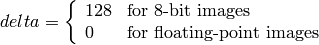
- lo_diff (CvScalar) – Maximal lower brightness/color difference between the currently observed pixel and one of its neighbors belonging to the component, or a seed pixel being added to the component. In the case of 8-bit color images it is a packed value
- up_diff (CvScalar) – Maximal upper brightness/color difference between the currently observed pixel and one of its neighbors belonging to the component, or a seed pixel being added to the component. In the case of 8-bit color images it is a packed value
- comp (CvConnectedComp) – Returned connected component for the repainted domain. Note that the function does not fill comp->contour field. The boundary of the filled component can be retrieved from the output mask image using FindContours
- flags (int) –
The operation flags. Lower bits contain connectivity value, 4 (by default) or 8, used within the function. Connectivity determines which neighbors of a pixel are considered. Upper bits can be 0 or a combination of the following flags:
- CV_FLOODFILL_FIXED_RANGE if set, the difference between the current pixel and seed pixel is considered, otherwise the difference between neighbor pixels is considered (the range is floating)
- CV_FLOODFILL_MASK_ONLY if set, the function does not fill the image ( new_val is ignored), but fills the mask (that must be non-NULL in this case)
- mask (CvArr) – Operation mask, should be a single-channel 8-bit image, 2 pixels wider and 2 pixels taller than image . If not NULL, the function uses and updates the mask, so the user takes responsibility of initializing the mask content. Floodfilling can’t go across non-zero pixels in the mask, for example, an edge detector output can be used as a mask to stop filling at edges. It is possible to use the same mask in multiple calls to the function to make sure the filled area do not overlap. Note : because the mask is larger than the filled image, a pixel in mask that corresponds to
 pixel in image will have coordinates
The function fills a connected component starting from the seed point with the specified color. The connectivity is determined by the closeness of pixel values. The pixel at
is considered to belong to the repainted domain if:
grayscale image, floating range

grayscale image, fixed range

color image, floating range


color image, fixed range


where
 is the value of one of pixel neighbors. That is, to be added to the connected component, a pixel’s color/brightness should be close enough to the:
- color/brightness of one of its neighbors that are already referred to the connected component in the case of floating range
- color/brightness of the seed point in the case of fixed range.
Inpaint
- Inpaint(src, mask, dst, inpaintRadius, flags) → None
Inpaints the selected region in the image.
Parameters: - src (CvArr) – The input 8-bit 1-channel or 3-channel image.
- mask (CvArr) – The inpainting mask, 8-bit 1-channel image. Non-zero pixels indicate the area that needs to be inpainted.
- dst (CvArr) – The output image of the same format and the same size as input.
- inpaintRadius (float) – The radius of circlular neighborhood of each point inpainted that is considered by the algorithm.
- flags (int) –
The inpainting method, one of the following:
- CV_INPAINT_NS Navier-Stokes based method.
- CV_INPAINT_TELEA The method by Alexandru Telea Telea04
The function reconstructs the selected image area from the pixel near the area boundary. The function may be used to remove dust and scratches from a scanned photo, or to remove undesirable objects from still images or video.
Integral
- Integral(image, sum, sqsum=NULL, tiltedSum=NULL) → None
Calculates the integral of an image.
Parameters: - image (CvArr) – The source image,
 , 8-bit or floating-point (32f or 64f)
 - sum (CvArr) – The integral image,
 , 32-bit integer or double precision floating-point (64f)
 - sqsum (CvArr) – The integral image for squared pixel values, , double precision floating-point (64f)
- tiltedSum (CvArr) – The integral for the image rotated by 45 degrees, , the same data type as sum
- image (CvArr) – The source image,
The function calculates one or more integral images for the source image as following:
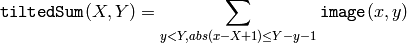
Using these integral images, one may calculate sum, mean and standard deviation over a specific up-right or rotated rectangular region of the image in a constant time, for example:

It makes possible to do a fast blurring or fast block correlation with variable window size, for example. In the case of multi-channel images, sums for each channel are accumulated independently.
PyrMeanShiftFiltering
- PyrMeanShiftFiltering(src, dst, sp, sr, max_level=1, termcrit=(CV_TERMCRIT_ITER+CV_TERMCRIT_EPS, 5, 1)) → None
Does meanshift image segmentation
Parameters: - src (CvArr) – The source 8-bit, 3-channel image.
- dst (CvArr) – The destination image of the same format and the same size as the source.
- sp (float) – The spatial window radius.
- sr (float) – The color window radius.
- max_level (int) – Maximum level of the pyramid for the segmentation.
- termcrit (CvTermCriteria) – Termination criteria: when to stop meanshift iterations.
The function implements the filtering
stage of meanshift segmentation, that is, the output of the function is
the filtered “posterized” image with color gradients and fine-grain
texture flattened. At every pixel
 of the input image (or
down-sized input image, see below) the function executes meanshift
iterations, that is, the pixel
neighborhood in the joint
space-color hyperspace is considered:
of the input image (or
down-sized input image, see below) the function executes meanshift
iterations, that is, the pixel
neighborhood in the joint
space-color hyperspace is considered:

where (R,G,B) and (r,g,b) are the vectors of color components at (X,Y) and (x,y) , respectively (though, the algorithm does not depend on the color space used, so any 3-component color space can be used instead). Over the neighborhood the average spatial value (X',Y') and average color vector (R',G',B') are found and they act as the neighborhood center on the next iteration:
 After the iterations over, the color components of the initial pixel (that is, the pixel from where the iterations started) are set to the final value (average color at the last iteration):
 Then
Then
 , the gaussian pyramid of
 levels is built, and the above procedure is run
on the smallest layer. After that, the results are propagated to the
larger layer and the iterations are run again only on those pixels where
the layer colors differ much (
levels is built, and the above procedure is run
on the smallest layer. After that, the results are propagated to the
larger layer and the iterations are run again only on those pixels where
the layer colors differ much (
 ) from the lower-resolution
layer, that is, the boundaries of the color regions are clarified. Note,
that the results will be actually different from the ones obtained by
running the meanshift procedure on the whole original image (i.e. when
) from the lower-resolution
layer, that is, the boundaries of the color regions are clarified. Note,
that the results will be actually different from the ones obtained by
running the meanshift procedure on the whole original image (i.e. when
 ).
).
PyrSegmentation
- PyrSegmentation(src, dst, storage, level, threshold1, threshold2) → comp
Implements image segmentation by pyramids.
Parameters: - src (IplImage) – The source image
- dst (IplImage) – The destination image
- storage (CvMemStorage) – Storage; stores the resulting sequence of connected components
- comp (CvSeq) – Pointer to the output sequence of the segmented components
- level (int) – Maximum level of the pyramid for the segmentation
- threshold1 (float) – Error threshold for establishing the links
- threshold2 (float) – Error threshold for the segments clustering
The function implements image segmentation by pyramids. The pyramid builds up to the level
level
. The links between any pixel
a
on level
i
and its candidate father pixel
b
on the adjacent level are established if
 .
After the connected components are defined, they are joined into several clusters.
Any two segments A and B belong to the same cluster, if
.
After the connected components are defined, they are joined into several clusters.
Any two segments A and B belong to the same cluster, if
 .
If the input image has only one channel, then
.
If the input image has only one channel, then
 .
If the input image has three channels (red, green and blue), then
.
If the input image has three channels (red, green and blue), then

There may be more than one connected component per a cluster. The images src and dst should be 8-bit single-channel or 3-channel images or equal size.
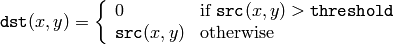
Threshold
- Threshold(src, dst, threshold, maxValue, thresholdType) → None
Applies a fixed-level threshold to array elements.
Parameters: - src (CvArr) – Source array (single-channel, 8-bit or 32-bit floating point)
- dst (CvArr) – Destination array; must be either the same type as src or 8-bit
- threshold (float) – Threshold value
- maxValue (float) – Maximum value to use with CV_THRESH_BINARY and CV_THRESH_BINARY_INV thresholding types
- thresholdType (int) – Thresholding type (see the discussion)
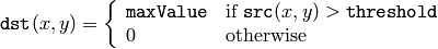
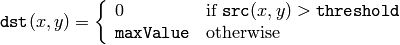
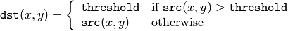
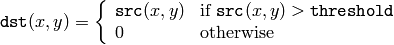
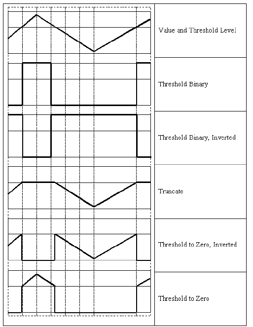
The function applies fixed-level thresholding to a single-channel array. The function is typically used to get a bi-level (binary) image out of a grayscale image ( CmpS could be also used for this purpose) or for removing a noise, i.e. filtering out pixels with too small or too large values. There are several types of thresholding that the function supports that are determined by thresholdType :
CV_THRESH_BINARY
CV_THRESH_BINARY_INV
CV_THRESH_TRUNC
CV_THRESH_TOZERO
CV_THRESH_TOZERO_INV
Also, the special value CV_THRESH_OTSU may be combined with one of the above values. In this case the function determines the optimal threshold value using Otsu’s algorithm and uses it instead of the specified thresh . The function returns the computed threshold value. Currently, Otsu’s method is implemented only for 8-bit images.
Help and Feedback
You did not find what you were looking for?- Try the Cookbook.
- Ask a question in the user group/mailing list.
- If you think something is missing or wrong in the documentation, please file a bug report.