Histograms

cv::calcHist

Comments from the Wiki

void calcHist(const Mat* arrays, int narrays, const int* channels, const Mat& mask, MatND& hist, int dims, const int* histSize, const float** ranges, bool uniform=true, bool accumulate=false)

void calcHist(const Mat* arrays, int narrays, const int* channels, const Mat& mask, SparseMat& hist, int dims, const int* histSize, const float** ranges, bool uniform=true, bool accumulate=false)

Calculates histogram of a set of arrays

Parameters:

• arrays – Source arrays. They all should have the same depth, CV_8U or CV_32F , and the same size. Each of them can have an arbitrary number of channels
• narrays – The number of source arrays
• channels – The list of dims channels that are used to compute the histogram. The first array channels are numerated from 0 to arrays[0].channels()-1 , the second array channels are counted from arrays[0].channels() to arrays[0].channels() + arrays[1].channels()-1 etc.
• mask – The optional mask. If the matrix is not empty, it must be 8-bit array of the same size as arrays[i] . The non-zero mask elements mark the array elements that are counted in the histogram
• hist – The output histogram, a dense or sparse dims -dimensional array
• dims – The histogram dimensionality; must be positive and not greater than CV_MAX_DIMS (=32 in the current OpenCV version)
• histSize – The array of histogram sizes in each dimension
• ranges – The array of dims arrays of the histogram bin boundaries in each dimension. When the histogram is uniform ( uniform =true), then for each dimension i it’s enough to specify the lower (inclusive) boundary of the 0-th histogram bin and the upper (exclusive) boundary for the last histogram bin histSize[i]-1 . That is, in the case of uniform histogram each of ranges[i] is an array of 2 elements. When the histogram is not uniform ( uniform=false ), then each of ranges[i] contains histSize[i]+1 elements: . The array elements, which are not between and , are not counted in the histogram
• uniform – Indicates whether the histogram is uniform or not, see above
• accumulate – Accumulation flag. If it is set, the histogram is not cleared in the beginning (when it is allocated). This feature allows user to compute a single histogram from several sets of arrays, or to update the histogram in time

The functions calcHist calculate the histogram of one or more arrays. The elements of a tuple that is used to increment a histogram bin are taken at the same location from the corresponding input arrays. The sample below shows how to compute 2D Hue-Saturation histogram for a color imag

#include <cv.h>
#include <highgui.h>

using namespace cv;

int main( int argc, char** argv )
{
    Mat src, hsv;
    if( argc != 2 || !(src=imread(argv[1], 1)).data )
        return -1;

    cvtColor(src, hsv, CV_BGR2HSV);

    // let's quantize the hue to 30 levels
    // and the saturation to 32 levels
    int hbins = 30, sbins = 32;
    int histSize[] = {hbins, sbins};
    // hue varies from 0 to 179, see cvtColor
    float hranges[] = { 0, 180 };
    // saturation varies from 0 (black-gray-white) to
    // 255 (pure spectrum color)
    float sranges[] = { 0, 256 };
    const float* ranges[] = { hranges, sranges };
    MatND hist;
    // we compute the histogram from the 0-th and 1-st channels
    int channels[] = {0, 1};

    calcHist( &hsv, 1, channels, Mat(), // do not use mask
             hist, 2, histSize, ranges,
             true, // the histogram is uniform
             false );
    double maxVal=0;
    minMaxLoc(hist, 0, &maxVal, 0, 0);

    int scale = 10;
    Mat histImg = Mat::zeros(sbins*scale, hbins*10, CV_8UC3);

    for( int h = 0; h < hbins; h++ )
        for( int s = 0; s < sbins; s++ )
        {
            float binVal = hist.at<float>(h, s);
            int intensity = cvRound(binVal*255/maxVal);
            rectangle( histImg, Point(h*scale, s*scale),
                        Point( (h+1)*scale - 1, (s+1)*scale - 1),
                        Scalar::all(intensity),
                        CV_FILLED );
        }

    namedWindow( "Source", 1 );
    imshow( "Source", src );

    namedWindow( "H-S Histogram", 1 );
    imshow( "H-S Histogram", histImg );
    waitKey();
}

cv::calcBackProject

Comments from the Wiki

void calcBackProject(const Mat* arrays, int narrays, const int* channels, const MatND& hist, Mat& backProject, const float** ranges, double scale=1, bool uniform=true)

void calcBackProject(const Mat* arrays, int narrays, const int* channels, const SparseMat& hist, Mat& backProject, const float** ranges, double scale=1, bool uniform=true)

Calculates the back projection of a histogram.

Parameters:

• arrays – Source arrays. They all should have the same depth, CV_8U or CV_32F , and the same size. Each of them can have an arbitrary number of channels
• narrays – The number of source arrays
• channels – The list of channels that are used to compute the back projection. The number of channels must match the histogram dimensionality. The first array channels are numerated from 0 to arrays[0].channels()-1 , the second array channels are counted from arrays[0].channels() to arrays[0].channels() + arrays[1].channels()-1 etc.
• hist – The input histogram, a dense or sparse
• backProject – Destination back projection aray; will be a single-channel array of the same size and the same depth as arrays[0]
• ranges – The array of arrays of the histogram bin boundaries in each dimension. See calcHist()
• scale – The optional scale factor for the output back projection
• uniform – Indicates whether the histogram is uniform or not, see above

The functions calcBackProject calculate the back project of the histogram. That is, similarly to calcHist , at each location (x, y) the function collects the values from the selected channels in the input images and finds the corresponding histogram bin. But instead of incrementing it, the function reads the bin value, scales it by scale and stores in backProject(x,y) . In terms of statistics, the function computes probability of each element value in respect with the empirical probability distribution represented by the histogram. Here is how, for example, you can find and track a bright-colored object in a scene:

1. Before the tracking, show the object to the camera such that covers almost the whole frame. Calculate a hue histogram. The histogram will likely have a strong maximums, corresponding to the dominant colors in the object.
2. During the tracking, calculate back projection of a hue plane of each input video frame using that pre-computed histogram. Threshold the back projection to suppress weak colors. It may also have sense to suppress pixels with non sufficient color saturation and too dark or too bright pixels.
3. Find connected components in the resulting picture and choose, for example, the largest component.

That is the approximate algorithm of CAMShift() color object tracker.

See also: calcHist()

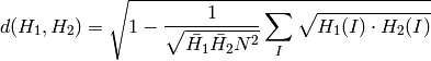
cv::compareHist

Comments from the Wiki

double compareHist(const MatND& H1, const MatND& H2, int method)

double compareHist(const SparseMat& H1, const SparseMat& H2, int method)

Compares two histograms

Parameters:

• H1 – The first compared histogram
• H2 – The second compared histogram of the same size as H1
• method –

  The comparison method, one of the following:

  • CV_COMP_CORREL Correlation
  • CV_COMP_CHISQR Chi-Square
  • CV_COMP_INTERSECT Intersection
  • CV_COMP_BHATTACHARYYA Bhattacharyya distance

The functions compareHist compare two dense or two sparse histograms using the specified method:

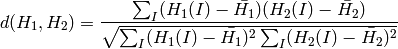
• Correlation (method=CV_COMP_CORREL)

  

  where

  

  and is the total number of histogram bins.

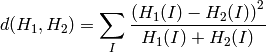
• Chi-Square (method=CV_COMP_CHISQR)

  

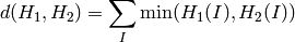
• Intersection (method=CV_COMP_INTERSECT)

  

• Bhattacharyya distance (method=CV_COMP_BHATTACHARYYA)

  

The function returns .

While the function works well with 1-, 2-, 3-dimensional dense histograms, it may not be suitable for high-dimensional sparse histograms, where, because of aliasing and sampling problems the coordinates of non-zero histogram bins can slightly shift. To compare such histograms or more general sparse configurations of weighted points, consider using the calcEMD() function.

cv::equalizeHist

Comments from the Wiki

void equalizeHist(const Mat& src, Mat& dst)

Equalizes the histogram of a grayscale image.

Parameters:

• src – The source 8-bit single channel image
• dst – The destination image; will have the same size and the same type as src

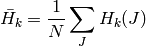
The function equalizes the histogram of the input image using the following algorithm:

1. calculate the histogram for src .

2. normalize the histogram so that the sum of histogram bins is 255.

3. compute the integral of the histogram:

   

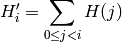
4. transform the image using as a look-up table:

The algorithm normalizes the brightness and increases the contrast of the image.