Neural Networks

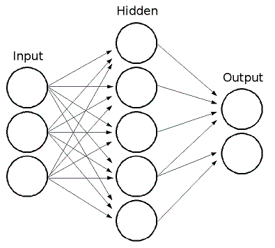
ML implements feed-forward artificial neural networks, more particularly, multi-layer perceptrons (MLP), the most commonly used type of neural networks. MLP consists of the input layer, output layer and one or more hidden layers. Each layer of MLP includes one or more neurons that are directionally linked with the neurons from the previous and the next layer. Here is an example of a 3-layer perceptron with 3 inputs, 2 outputs and the hidden layer including 5 neurons:

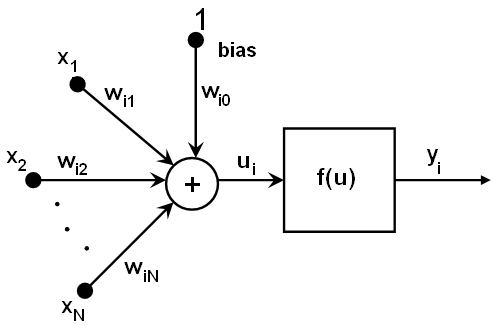
All the neurons in MLP are similar. Each of them has several input links (i.e. it takes the output values from several neurons in the previous layer on input) and several output links (i.e. it passes the response to several neurons in the next layer). The values retrieved from the previous layer are summed with certain weights, individual for each neuron, plus the bias term, and the sum is transformed using the activation function that may be also different for different neurons. Here is the picture:

In other words, given the outputs of the layer , the outputs of the layer are computed as:

Different activation functions may be used, ML implements 3 standard ones:

• Identity function ( CvANN_MLP::IDENTITY ):

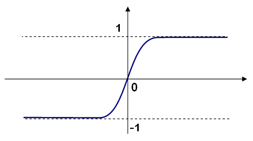
• Symmetrical sigmoid ( CvANN_MLP::SIGMOID_SYM ): ), the default choice for MLP; the standard sigmoid with is shown below:

  

• Gaussian function ( CvANN_MLP::GAUSSIAN ): , not completely supported by the moment.

In ML all the neurons have the same activation functions, with the same free parameters ( ) that are specified by user and are not altered by the training algorithms.

So the whole trained network works as follows: It takes the feature vector on input, the vector size is equal to the size of the input layer, when the values are passed as input to the first hidden layer, the outputs of the hidden layer are computed using the weights and the activation functions and passed further downstream, until we compute the output layer.

So, in order to compute the network one needs to know all the weights . The weights are computed by the training algorithm. The algorithm takes a training set: multiple input vectors with the corresponding output vectors, and iteratively adjusts the weights to try to make the network give the desired response on the provided input vectors.

The larger the network size (the number of hidden layers and their sizes), the more is the potential network flexibility, and the error on the training set could be made arbitrarily small. But at the same time the learned network will also “learn” the noise present in the training set, so the error on the test set usually starts increasing after the network size reaches some limit. Besides, the larger networks are train much longer than the smaller ones, so it is reasonable to preprocess the data (using CalcPCA or similar technique) and train a smaller network on only the essential features.

Another feature of the MLP’s is their inability to handle categorical data as is, however there is a workaround. If a certain feature in the input or output (i.e. in the case of n -class classifier for ) layer is categorical and can take different values, it makes sense to represent it as binary tuple of M elements, where i -th element is 1 if and only if the feature is equal to the i -th value out of M possible. It will increase the size of the input/output layer, but will speedup the training algorithm convergence and at the same time enable “fuzzy” values of such variables, i.e. a tuple of probabilities instead of a fixed value.

ML implements 2 algorithms for training MLP’s. The first is the classical random sequential back-propagation algorithm and the second (default one) is batch RPROP algorithm.

References:

• http://en.wikipedia.org/wiki/Backpropagation . Wikipedia article about the back-propagation algorithm.
• 25. LeCun, L. Bottou, G.B. Orr and K.-R. Muller, “Efficient backprop”, in Neural Networks—Tricks of the Trade, Springer Lecture Notes in Computer Sciences 1524, pp.5-50, 1998.
• 13. Riedmiller and H. Braun, “A Direct Adaptive Method for Faster Backpropagation Learning: The RPROP Algorithm”, Proc. ICNN, San Francisco (1993).

CvANN_MLP_TrainParams

Comments from the Wiki

CvANN_MLP_TrainParams

Parameters of the MLP training algorithm.

struct CvANN_MLP_TrainParams
{
    CvANN_MLP_TrainParams();
    CvANN_MLP_TrainParams( CvTermCriteria term_crit, int train_method,
                           double param1, double param2=0 );
    ~CvANN_MLP_TrainParams();

    enum { BACKPROP=0, RPROP=1 };

    CvTermCriteria term_crit;
    int train_method;

    // backpropagation parameters
    double bp_dw_scale, bp_moment_scale;

    // rprop parameters
    double rp_dw0, rp_dw_plus, rp_dw_minus, rp_dw_min, rp_dw_max;
};

The structure has default constructor that initializes parameters for RPROP algorithm. There is also more advanced constructor to customize the parameters and/or choose backpropagation algorithm. Finally, the individual parameters can be adjusted after the structure is created.

CvANN_MLP

Comments from the Wiki

CvANN_MLP

MLP model.

class CvANN_MLP : public CvStatModel
{
public:
    CvANN_MLP();
    CvANN_MLP( const CvMat* _layer_sizes,
               int _activ_func=SIGMOID_SYM,
               double _f_param1=0, double _f_param2=0 );

    virtual ~CvANN_MLP();

    virtual void create( const CvMat* _layer_sizes,
                         int _activ_func=SIGMOID_SYM,
                         double _f_param1=0, double _f_param2=0 );

    virtual int train( const CvMat* _inputs, const CvMat* _outputs,
                       const CvMat* _sample_weights,
                       const CvMat* _sample_idx=0,
                       CvANN_MLP_TrainParams _params = CvANN_MLP_TrainParams(),
                       int flags=0 );
    virtual float predict( const CvMat* _inputs,
                           CvMat* _outputs ) const;

    virtual void clear();

    // possible activation functions
    enum { IDENTITY = 0, SIGMOID_SYM = 1, GAUSSIAN = 2 };

    // available training flags
    enum { UPDATE_WEIGHTS = 1, NO_INPUT_SCALE = 2, NO_OUTPUT_SCALE = 4 };

    virtual void read( CvFileStorage* fs, CvFileNode* node );
    virtual void write( CvFileStorage* storage, const char* name );

    int get_layer_count() { return layer_sizes ? layer_sizes->cols : 0; }
    const CvMat* get_layer_sizes() { return layer_sizes; }

protected:

    virtual bool prepare_to_train( const CvMat* _inputs, const CvMat* _outputs,
            const CvMat* _sample_weights, const CvMat* _sample_idx,
            CvANN_MLP_TrainParams _params,
            CvVectors* _ivecs, CvVectors* _ovecs, double** _sw, int _flags );

    // sequential random backpropagation
    virtual int train_backprop( CvVectors _ivecs, CvVectors _ovecs,
                                                const double* _sw );

    // RPROP algorithm
    virtual int train_rprop( CvVectors _ivecs, CvVectors _ovecs,
                                             const double* _sw );

    virtual void calc_activ_func( CvMat* xf, const double* bias ) const;
    virtual void calc_activ_func_deriv( CvMat* xf, CvMat* deriv,
                                             const double* bias ) const;
    virtual void set_activ_func( int _activ_func=SIGMOID_SYM,
                                 double _f_param1=0, double _f_param2=0 );
    virtual void init_weights();
    virtual void scale_input( const CvMat* _src, CvMat* _dst ) const;
    virtual void scale_output( const CvMat* _src, CvMat* _dst ) const;
    virtual void calc_input_scale( const CvVectors* vecs, int flags );
    virtual void calc_output_scale( const CvVectors* vecs, int flags );

    virtual void write_params( CvFileStorage* fs );
    virtual void read_params( CvFileStorage* fs, CvFileNode* node );

    CvMat* layer_sizes;
    CvMat* wbuf;
    CvMat* sample_weights;
    double** weights;
    double f_param1, f_param2;
    double min_val, max_val, min_val1, max_val1;
    int activ_func;
    int max_count, max_buf_sz;
    CvANN_MLP_TrainParams params;
    CvRNG rng;
};

Unlike many other models in ML that are constructed and trained at once, in the MLP model these steps are separated. First, a network with the specified topology is created using the non-default constructor or the method create . All the weights are set to zeros. Then the network is trained using the set of input and output vectors. The training procedure can be repeated more than once, i.e. the weights can be adjusted based on the new training data.

CvANN_MLP::create

Comments from the Wiki

void CvANN_MLP::create(const CvMat* _layer_sizes, int _activ_func=SIGMOID_SYM, double _f_param1=0, double _f_param2=0)

Constructs the MLP with the specified topology

Parameters:

• _layer_sizes – The integer vector specifies the number of neurons in each layer including the input and output layers.
• _activ_func – Specifies the activation function for each neuron; one of CvANN_MLP::IDENTITY , CvANN_MLP::SIGMOID_SYM and CvANN_MLP::GAUSSIAN .
• _f_param1,_f_param2 – Free parameters of the activation function, and , respectively. See the formulas in the introduction section.

The method creates a MLP network with the specified topology and assigns the same activation function to all the neurons.

CvANN_MLP::train

Comments from the Wiki

int CvANN_MLP::train(const CvMat* _inputs, const CvMat* _outputs, const CvMat* _sample_weights, const CvMat* _sample_idx=0, CvANN_MLP_TrainParams _params = CvANN_MLP_TrainParams(), int flags=0)

Trains/updates MLP.

Parameters:

• _inputs – A floating-point matrix of input vectors, one vector per row.
• _outputs – A floating-point matrix of the corresponding output vectors, one vector per row.
• _sample_weights – (RPROP only) The optional floating-point vector of weights for each sample. Some samples may be more important than others for training, and the user may want to raise the weight of certain classes to find the right balance between hit-rate and false-alarm rate etc.
• _sample_idx – The optional integer vector indicating the samples (i.e. rows of _inputs and _outputs ) that are taken into account.
• _params – The training params. See CvANN_MLP_TrainParams description.
• _flags –

  The various parameters to control the training algorithm. May be a combination of the following:

  • UPDATE_WEIGHTS = 1 algorithm updates the network weights, rather than computes them from scratch (in the latter case the weights are initialized using Nguyen-Widrow algorithm).
  • NO_INPUT_SCALE algorithm does not normalize the input vectors. If this flag is not set, the training algorithm normalizes each input feature independently, shifting its mean value to 0 and making the standard deviation =1. If the network is assumed to be updated frequently, the new training data could be much different from original one. In this case user should take care of proper normalization.
  • NO_OUTPUT_SCALE algorithm does not normalize the output vectors. If the flag is not set, the training algorithm normalizes each output features independently, by transforming it to the certain range depending on the activation function used.

This method applies the specified training algorithm to compute/adjust the network weights. It returns the number of done iterations.