Structural Analysis and Shape Descriptors
ApproxChains
- ApproxChains(src_seq, storage, method=CV_CHAIN_APPROX_SIMPLE, parameter=0, minimal_perimeter=0, recursive=0) → chains
Approximates Freeman chain(s) with a polygonal curve.
Parameters: - src_seq (CvSeq) – Pointer to the chain that can refer to other chains
- storage (CvMemStorage) – Storage location for the resulting polylines
- method (int) – Approximation method (see the description of the function FindContours )
- parameter (float) – Method parameter (not used now)
- minimal_perimeter (int) – Approximates only those contours whose perimeters are not less than minimal_perimeter . Other chains are removed from the resulting structure
- recursive (int) – If not 0, the function approximates all chains that access can be obtained to from src_seq by using the h_next or v_next links . If 0, the single chain is approximated
This is a stand-alone approximation routine. The function cvApproxChains works exactly in the same way as FindContours with the corresponding approximation flag. The function returns pointer to the first resultant contour. Other approximated contours, if any, can be accessed via the v_next or h_next fields of the returned structure.
ApproxPoly
ApproxPoly(src_seq, storage, method, parameter=0, parameter2=0) -> sequence
Approximates polygonal curve(s) with the specified precision.
param src_seq: Sequence of an array of points type src_seq: CvArr or CvSeq param storage: Container for the approximated contours. If it is NULL, the input sequences’ storage is used type storage: CvMemStorage param method: Approximation method; only CV_POLY_APPROX_DP is supported, that corresponds to the Douglas-Peucker algorithm type method: int param parameter: Method-specific parameter; in the case of CV_POLY_APPROX_DP it is a desired approximation accuracy type parameter: float param parameter2: If case if src_seq is a sequence, the parameter determines whether the single sequence should be approximated or all sequences on the same level or below src_seq (see FindContours for description of hierarchical contour structures). If src_seq is an array CvMat* of points, the parameter specifies whether the curve is closed ( parameter2 !=0) or not ( parameter2 =0) type parameter2: int
The function approximates one or more curves and returns the approximation result[s]. In the case of multiple curves, the resultant tree will have the same structure as the input one (1:1 correspondence).
ArcLength
- ArcLength(curve, slice=CV_WHOLE_SEQ, isClosed=-1) → double
Calculates the contour perimeter or the curve length.
Parameters: - curve (CvArr or CvSeq) – Sequence or array of the curve points
- slice (CvSlice) – Starting and ending points of the curve, by default, the whole curve length is calculated
- isClosed (int) –
Indicates whether the curve is closed or not. There are 3 cases:
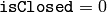 the curve is assumed to be unclosed.
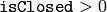 the curve is assumed to be closed.
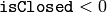 if curve is sequence, the flag CV_SEQ_FLAG_CLOSED of ((CvSeq*)curve)->flags is checked to determine if the curve is closed or not, otherwise (curve is represented by array (CvMat*) of points) it is assumed to be unclosed.
The function calculates the length or curve as the sum of lengths of segments between subsequent points
BoundingRect
- BoundingRect(points, update=0) → CvRect
Calculates the up-right bounding rectangle of a point set.
Parameters:
The function returns the up-right bounding rectangle for a 2d point set. Here is the list of possible combination of the flag values and type of points :
| update | points | action |
|---|---|---|
| 0 | CvContour* | the bounding rectangle is not calculated, but it is taken from rect field of the contour header. |
| 1 | CvContour* | the bounding rectangle is calculated and written to rect field of the contour header. |
| 0 | CvSeq* or CvMat* | the bounding rectangle is calculated and returned. |
| 1 | CvSeq* or CvMat* | runtime error is raised. |
BoxPoints
- BoxPoints(box) → points
Finds the box vertices.
Parameters: - box (CvBox2D) – Box
- points (CvPoint2D32f_4) – Array of vertices
The function calculates the vertices of the input 2d box.
CalcPGH
- CalcPGH(contour, hist) → None
Calculates a pair-wise geometrical histogram for a contour.
Parameters: - contour – Input contour. Currently, only integer point coordinates are allowed
- hist – Calculated histogram; must be two-dimensional
The function calculates a 2D pair-wise geometrical histogram (PGH), described in Iivarinen97 for the contour. The algorithm considers every pair of contour edges. The angle between the edges and the minimum/maximum distances are determined for every pair. To do this each of the edges in turn is taken as the base, while the function loops through all the other edges. When the base edge and any other edge are considered, the minimum and maximum distances from the points on the non-base edge and line of the base edge are selected. The angle between the edges defines the row of the histogram in which all the bins that correspond to the distance between the calculated minimum and maximum distances are incremented (that is, the histogram is transposed relatively to the Iivarninen97 definition). The histogram can be used for contour matching.
CalcEMD2
- CalcEMD2(signature1, signature2, distance_type, distance_func = None, cost_matrix=None, flow=None, lower_bound=None, userdata = None) → float
Computes the “minimal work” distance between two weighted point configurations.
Parameters: - signature1 (CvArr) – First signature, a
 floating-point matrix. Each row stores the point weight followed by the point coordinates. The matrix is allowed to have a single column (weights only) if the user-defined cost matrix is used
 - signature2 (CvArr) – Second signature of the same format as signature1 , though the number of rows may be different. The total weights may be different, in this case an extra “dummy” point is added to either signature1 or signature2
- distance_type (int) – Metrics used; CV_DIST_L1, CV_DIST_L2 , and CV_DIST_C stand for one of the standard metrics; CV_DIST_USER means that a user-defined function distance_func or pre-calculated cost_matrix is used
- distance_func (PyCallableObject) – The user-supplied distance function. It takes coordinates of two points pt0 and pt1 , and returns the distance between the points, with sigature `` func(pt0, pt1, userdata) -> float``
- cost_matrix (CvArr) – The user-defined
 cost matrix. At least one of cost_matrix and distance_func must be NULL. Also, if a cost matrix is used, lower boundary (see below) can not be calculated, because it needs a metric function
 - flow (CvArr) – The resultant
 flow matrix:
  is a flow from
  th point of signature1 to
  th point of signature2
 - lower_bound (float) – Optional input/output parameter: lower boundary of distance between the two signatures that is a distance between mass centers. The lower boundary may not be calculated if the user-defined cost matrix is used, the total weights of point configurations are not equal, or if the signatures consist of weights only (i.e. the signature matrices have a single column). The user must initialize *lower_bound . If the calculated distance between mass centers is greater or equal to *lower_bound (it means that the signatures are far enough) the function does not calculate EMD. In any case *lower_bound is set to the calculated distance between mass centers on return. Thus, if user wants to calculate both distance between mass centers and EMD, *lower_bound should be set to 0
- userdata (object) – Pointer to optional data that is passed into the user-defined distance function
- signature1 (CvArr) – First signature, a
The function computes the earth mover distance and/or a lower boundary of the distance between the two weighted point configurations. One of the applications described in RubnerSept98 is multi-dimensional histogram comparison for image retrieval. EMD is a a transportation problem that is solved using some modification of a simplex algorithm, thus the complexity is exponential in the worst case, though, on average it is much faster. In the case of a real metric the lower boundary can be calculated even faster (using linear-time algorithm) and it can be used to determine roughly whether the two signatures are far enough so that they cannot relate to the same object.
CheckContourConvexity
- CheckContourConvexity(contour) → int
Tests contour convexity.
Parameters: contour (CvArr or CvSeq) – Tested contour (sequence or array of points)
The function tests whether the input contour is convex or not. The contour must be simple, without self-intersections.
CvConvexityDefect
- class CvConvexityDefect
A single contour convexity defect, represented by a tuple (start, end, depthpoint, depth) .
ContourArea
- ContourArea(contour, slice=CV_WHOLE_SEQ) → double
Calculates the area of a whole contour or a contour section.
Parameters:
The function calculates the area of a whole contour or a contour section. In the latter case the total area bounded by the contour arc and the chord connecting the 2 selected points is calculated as shown on the picture below:
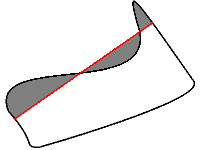
Orientation of the contour affects the area sign, thus the function may return a negative result. Use the fabs() function from C runtime to get the absolute value of the area.
ContourFromContourTree
- ContourFromContourTree(tree, storage, criteria) → contour
Restores a contour from the tree.
Parameters: - tree – Contour tree
- storage – Container for the reconstructed contour
- criteria – Criteria, where to stop reconstruction
The function restores the contour from its binary tree representation. The parameter criteria determines the accuracy and/or the number of tree levels used for reconstruction, so it is possible to build an approximated contour. The function returns the reconstructed contour.
ConvexHull2
- ConvexHull2(points, storage, orientation=CV_CLOCKWISE, return_points=0) → convex_hull
Finds the convex hull of a point set.
Parameters: - points (CvArr or CvSeq) – Sequence or array of 2D points with 32-bit integer or floating-point coordinates
- storage (CvMemStorage) – The destination array (CvMat*) or memory storage (CvMemStorage*) that will store the convex hull. If it is an array, it should be 1d and have the same number of elements as the input array/sequence. On output the header is modified as to truncate the array down to the hull size. If storage is NULL then the convex hull will be stored in the same storage as the input sequence
- orientation (int) – Desired orientation of convex hull: CV_CLOCKWISE or CV_COUNTER_CLOCKWISE
- return_points (int) – If non-zero, the points themselves will be stored in the hull instead of indices if storage is an array, or pointers if storage is memory storage
The function finds the convex hull of a 2D point set using Sklansky’s algorithm. If storage is memory storage, the function creates a sequence containing the hull points or pointers to them, depending on return_points value and returns the sequence on output. If storage is a CvMat, the function returns NULL.
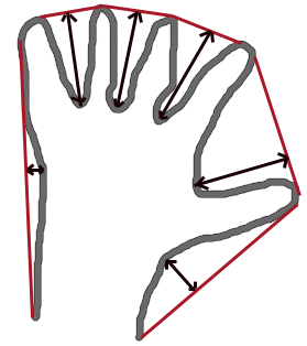
ConvexityDefects
- ConvexityDefects(contour, convexhull, storage) → convexity_defects
Finds the convexity defects of a contour.
Parameters: - contour (CvArr or CvSeq) – Input contour
- convexhull (CvSeq) – Convex hull obtained using ConvexHull2 that should contain pointers or indices to the contour points, not the hull points themselves (the return_points parameter in ConvexHull2 should be 0)
- storage (CvMemStorage) – Container for the output sequence of convexity defects. If it is NULL, the contour or hull (in that order) storage is used
The function finds all convexity defects of the input contour and returns a sequence of the CvConvexityDefect structures.
CreateContourTree
- CreateContourTree(contour, storage, threshold) → contour_tree
Creates a hierarchical representation of a contour.
Parameters: - contour – Input contour
- storage – Container for output tree
- threshold – Approximation accuracy
The function creates a binary tree representation for the input contour and returns the pointer to its root. If the parameter threshold is less than or equal to 0, the function creates a full binary tree representation. If the threshold is greater than 0, the function creates a representation with the precision threshold : if the vertices with the interceptive area of its base line are less than threshold , the tree should not be built any further. The function returns the created tree.
FindContours
- FindContours(image, storage, mode=CV_RETR_LIST, method=CV_CHAIN_APPROX_SIMPLE, offset=(0, 0)) → cvseq
Finds the contours in a binary image.
Parameters: - image (CvArr) – The source, an 8-bit single channel image. Non-zero pixels are treated as 1’s, zero pixels remain 0’s - the image is treated as binary . To get such a binary image from grayscale, one may use Threshold , AdaptiveThreshold or Canny . The function modifies the source image’s content
- storage (CvMemStorage) – Container of the retrieved contours
- mode (int) –
Retrieval mode
- CV_RETR_EXTERNAL retrives only the extreme outer contours
- CV_RETR_LIST retrieves all of the contours and puts them in the list
- CV_RETR_CCOMP retrieves all of the contours and organizes them into a two-level hierarchy: on the top level are the external boundaries of the components, on the second level are the boundaries of the holes
- CV_RETR_TREE retrieves all of the contours and reconstructs the full hierarchy of nested contours
- method (int) –
Approximation method (for all the modes, except CV_LINK_RUNS , which uses built-in approximation)
- CV_CHAIN_CODE outputs contours in the Freeman chain code. All other methods output polygons (sequences of vertices)
- CV_CHAIN_APPROX_NONE translates all of the points from the chain code into points
- CV_CHAIN_APPROX_SIMPLE compresses horizontal, vertical, and diagonal segments and leaves only their end points
- CV_CHAIN_APPROX_TC89_L1,CV_CHAIN_APPROX_TC89_KCOS applies one of the flavors of the Teh-Chin chain approximation algorithm.
- CV_LINK_RUNS uses a completely different contour retrieval algorithm by linking horizontal segments of 1’s. Only the CV_RETR_LIST retrieval mode can be used with this method.
- offset (CvPoint) – Offset, by which every contour point is shifted. This is useful if the contours are extracted from the image ROI and then they should be analyzed in the whole image context
The function retrieves contours from the binary image using the algorithm Suzuki85 . The contours are a useful tool for shape analysis and object detection and recognition.
The function retrieves contours from the binary image and returns the number of retrieved contours. The pointer first_contour is filled by the function. It will contain a pointer to the first outermost contour or NULL if no contours are detected (if the image is completely black). Other contours may be reached from first_contour using the h_next and v_next links. The sample in the DrawContours discussion shows how to use contours for connected component detection. Contours can be also used for shape analysis and object recognition - see squares.py in the OpenCV sample directory.
Note: the source image is modified by this function.
FitEllipse2
- FitEllipse2(points) → Box2D
Fits an ellipse around a set of 2D points.
Parameters: points (CvArr) – Sequence or array of points
The function calculates the ellipse that fits best (in least-squares sense) around a set of 2D points. The meaning of the returned structure fields is similar to those in Ellipse except that size stores the full lengths of the ellipse axises, not half-lengths.
FitLine
- FitLine(points, dist_type, param, reps, aeps) → line
Fits a line to a 2D or 3D point set.
Parameters: - points (CvArr) – Sequence or array of 2D or 3D points with 32-bit integer or floating-point coordinates
- dist_type (int) – The distance used for fitting (see the discussion)
- param (float) – Numerical parameter ( C ) for some types of distances, if 0 then some optimal value is chosen
- reps (float) – Sufficient accuracy for the radius (distance between the coordinate origin and the line). 0.01 is a good default value.
- aeps (float) – Sufficient accuracy for the angle. 0.01 is a good default value.
- line (object) – The output line parameters. In the case of a 2d fitting, it is a tuple of 4 floats (vx, vy, x0, y0) where (vx, vy) is a normalized vector collinear to the line and (x0, y0) is some point on the line. in the case of a 3D fitting it is a tuple of 6 floats (vx, vy, vz, x0, y0, z0) where (vx, vy, vz) is a normalized vector collinear to the line and (x0, y0, z0) is some point on the line
The function fits a line to a 2D or 3D point set by minimizing
 where
where
 is the distance between the
th point and the line and
is the distance between the
th point and the line and
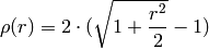
 is a distance function, one of:
dist_type=CV_DIST_L2

dist_type=CV_DIST_L1

dist_type=CV_DIST_L12
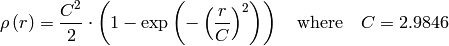
dist_type=CV_DIST_FAIR

dist_type=CV_DIST_WELSCH
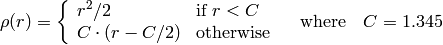
dist_type=CV_DIST_HUBER
GetCentralMoment
- GetCentralMoment(moments, x_order, y_order) → double
Retrieves the central moment from the moment state structure.
Parameters: - moments (CvMoments) – Pointer to the moment state structure
- x_order (int) – x order of the retrieved moment,
- y_order (int) – y order of the retrieved moment,
 and
and 
The function retrieves the central moment, which in the case of image moments is defined as:

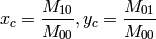
where
 are the coordinates of the gravity center:
GetHuMoments
- GetHuMoments(moments) → hu
Calculates the seven Hu invariants.
Parameters: - moments (CvMoments) – The input moments, computed with Moments
- hu (object) – The output Hu invariants
The function calculates the seven Hu invariants, see http://en.wikipedia.org/wiki/Image_moment , that are defined as:
![\begin{array}{l} hu_1= \eta _{20}+ \eta _{02} \\ hu_2=( \eta _{20}- \eta _{02})^{2}+4 \eta _{11}^{2} \\ hu_3=( \eta _{30}-3 \eta _{12})^{2}+ (3 \eta _{21}- \eta _{03})^{2} \\ hu_4=( \eta _{30}+ \eta _{12})^{2}+ ( \eta _{21}+ \eta _{03})^{2} \\ hu_5=( \eta _{30}-3 \eta _{12})( \eta _{30}+ \eta _{12})[( \eta _{30}+ \eta _{12})^{2}-3( \eta _{21}+ \eta _{03})^{2}]+(3 \eta _{21}- \eta _{03})( \eta _{21}+ \eta _{03})[3( \eta _{30}+ \eta _{12})^{2}-( \eta _{21}+ \eta _{03})^{2}] \\ hu_6=( \eta _{20}- \eta _{02})[( \eta _{30}+ \eta _{12})^{2}- ( \eta _{21}+ \eta _{03})^{2}]+4 \eta _{11}( \eta _{30}+ \eta _{12})( \eta _{21}+ \eta _{03}) \\ hu_7=(3 \eta _{21}- \eta _{03})( \eta _{21}+ \eta _{03})[3( \eta _{30}+ \eta _{12})^{2}-( \eta _{21}+ \eta _{03})^{2}]-( \eta _{30}-3 \eta _{12})( \eta _{21}+ \eta _{03})[3( \eta _{30}+ \eta _{12})^{2}-( \eta _{21}+ \eta _{03})^{2}] \\ \end{array}](_images/math/c0225e5b813ed803409286b71268108e4cceda75.png)
where
 denote the normalized central moments.
These values are proved to be invariant to the image scale, rotation, and reflection except the seventh one, whose sign is changed by reflection. Of course, this invariance was proved with the assumption of infinite image resolution. In case of a raster images the computed Hu invariants for the original and transformed images will be a bit different.
>>> import cv
>>> original = cv.LoadImageM("building.jpg", cv.CV_LOAD_IMAGE_GRAYSCALE)
>>> print cv.GetHuMoments(cv.Moments(original))
(0.0010620951868446141, 1.7962726159653835e-07, 1.4932744974469421e-11, 4.4832441315737963e-12, -1.0819359198251739e-23, -9.5726503811945833e-16, -3.5050592804744648e-23)
>>> flipped = cv.CloneMat(original)
>>> cv.Flip(original, flipped)
>>> print cv.GetHuMoments(cv.Moments(flipped))
(0.0010620951868446141, 1.796272615965384e-07, 1.4932744974469935e-11, 4.4832441315740249e-12, -1.0819359198259393e-23, -9.572650381193327e-16, 3.5050592804745877e-23)
GetNormalizedCentralMoment
- GetNormalizedCentralMoment(moments, x_order, y_order) → double
Retrieves the normalized central moment from the moment state structure.
Parameters: - moments (CvMoments) – Pointer to the moment state structure
- x_order (int) – x order of the retrieved moment,
- y_order (int) – y order of the retrieved moment, and
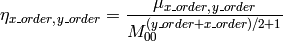
The function retrieves the normalized central moment:
GetSpatialMoment
- GetSpatialMoment(moments, x_order, y_order) → double
Retrieves the spatial moment from the moment state structure.
Parameters: - moments (CvMoments) – The moment state, calculated by Moments
- x_order (int) – x order of the retrieved moment,
- y_order (int) – y order of the retrieved moment, and
The function retrieves the spatial moment, which in the case of image moments is defined as:
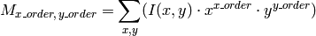
where
 is the intensity of the pixel
 .
.
MatchContourTrees
- MatchContourTrees(tree1, tree2, method, threshold) → double
Compares two contours using their tree representations.
Parameters: - tree1 – First contour tree
- tree2 – Second contour tree
- method – Similarity measure, only CV_CONTOUR_TREES_MATCH_I1 is supported
- threshold – Similarity threshold
The function calculates the value of the matching measure for two contour trees. The similarity measure is calculated level by level from the binary tree roots. If at a certain level the difference between contours becomes less than threshold , the reconstruction process is interrupted and the current difference is returned.
MatchShapes
- MatchShapes(object1, object2, method, parameter=0) → None
Compares two shapes.
Parameters:
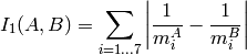
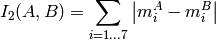
The function compares two shapes. The 3 implemented methods all use Hu moments (see
GetHuMoments
) (
 is
object1
,
is
object1
,
 is
object2
):
is
object2
):
method=CV_CONTOUR_MATCH_I1
method=CV_CONTOUR_MATCH_I2
method=CV_CONTOUR_MATCH_I3
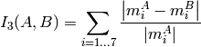
where

and
 are the Hu moments of
and
respectively.
are the Hu moments of
and
respectively.
MinAreaRect2
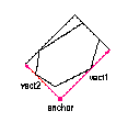
- MinAreaRect2(points, storage=NULL) → CvBox2D
Finds the circumscribed rectangle of minimal area for a given 2D point set.
Parameters: - points (CvArr or CvSeq) – Sequence or array of points
- storage (CvMemStorage) – Optional temporary memory storage
The function finds a circumscribed rectangle of the minimal area for a 2D point set by building a convex hull for the set and applying the rotating calipers technique to the hull.
Picture. Minimal-area bounding rectangle for contour
MinEnclosingCircle
- MinEnclosingCircle(points)-> (int, center, radius)
Finds the circumscribed circle of minimal area for a given 2D point set.
Parameters: - points (CvArr or CvSeq) – Sequence or array of 2D points
- center (CvPoint2D32f) – Output parameter; the center of the enclosing circle
- radius (float) – Output parameter; the radius of the enclosing circle
The function finds the minimal circumscribed circle for a 2D point set using an iterative algorithm. It returns nonzero if the resultant circle contains all the input points and zero otherwise (i.e. the algorithm failed).
Moments
- Moments(arr, binary = 0) → moments
Calculates all of the moments up to the third order of a polygon or rasterized shape.
Parameters: - arr (CvArr or CvSeq) – Image (1-channel or 3-channel with COI set) or polygon (CvSeq of points or a vector of points)
- moments (CvMoments) – Pointer to returned moment’s state structure
- binary (int) – (For images only) If the flag is non-zero, all of the zero pixel values are treated as zeroes, and all of the others are treated as 1’s
The function calculates spatial and central moments up to the third order and writes them to moments . The moments may then be used then to calculate the gravity center of the shape, its area, main axises and various shape characeteristics including 7 Hu invariants.
PointPolygonTest
- PointPolygonTest(contour, pt, measure_dist) → double
Point in contour test.
Parameters: - contour (CvArr or CvSeq) – Input contour
- pt (CvPoint2D32f) – The point tested against the contour
- measure_dist (int) – If it is non-zero, the function estimates the distance from the point to the nearest contour edge
The function determines whether the
point is inside a contour, outside, or lies on an edge (or coinsides
with a vertex). It returns positive, negative or zero value,
correspondingly. When
 , the return value
is +1, -1 and 0, respectively. When
, the return value
is +1, -1 and 0, respectively. When
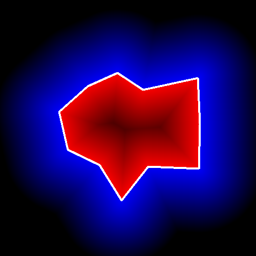
 ,
it is a signed distance between the point and the nearest contour
edge.
,
it is a signed distance between the point and the nearest contour
edge.
Here is the sample output of the function, where each image pixel is tested against the contour.
Help and Feedback
You did not find what you were looking for?- Try the Cookbook.
- Ask a question in the user group/mailing list.
- If you think something is missing or wrong in the documentation, please file a bug report.
![]()
Table Of Contents
- Structural Analysis and Shape Descriptors
- ApproxChains
- ApproxPoly
- ArcLength
- BoundingRect
- BoxPoints
- CalcPGH
- CalcEMD2
- CheckContourConvexity
- CvConvexityDefect
- ContourArea
- ContourFromContourTree
- ConvexHull2
- ConvexityDefects
- CreateContourTree
- FindContours
- FitEllipse2
- FitLine
- GetCentralMoment
- GetHuMoments
- GetNormalizedCentralMoment
- GetSpatialMoment
- MatchContourTrees
- MatchShapes
- MinAreaRect2
- MinEnclosingCircle
- Moments
- PointPolygonTest
Previous topic
Miscellaneous Image Transformations